

Digital signal processing
Digital signal processing (DSP) is the mathematical manipulation of an information signal to modify or improve it in some way. It is characterized by the representation of discrete time, discrete frequency, or other discrete domain signals by a sequence of numbers or symbols and the processing of these signals.
The goal of DSP is usually to measure, filter and/or compress continuous real-world analog signals. The first step is usually to convert the signal from an analog to a digital form, by sampling and then digitizing it using an analog-to-digital converter (ADC), which turns the analog signal into a stream of numbers. However, often, the required output signal is another analog output signal, which requires a digital-to-analog converter (DAC). Even if this process is more complex than analog processing and has a discrete value range, the application of computational power to digital signal processing allows for many advantages over analog processing in many applications, such as error detection and correction in transmission as well as data compression.
Digital signal processing and analog signal processing are subfields of signal processing. DSP applications include: audio and speech signal processing, sonar and radar signal processing, sensor array processing, spectral estimation, statistical signal processing, digital image processing, signal processing for communications, control of systems, biomedical signal processing, seismic data processing, etc. DSP algorithms have long been run on standard computers, as well as on specialized processors called digital signal processor and on purpose-built hardware such as application-specific integrated circuit (ASICs). Today there are additional technologies used for digital signal processing including more powerful general purpose microprocessors, field-programmable gate arrays (FPGAs), digital signal controllers (mostly for industrial apps such as motor control), and stream processors, among others.
Digital signal processing can involve linear or nonlinear operations. Nonlinear signal processing is closely related to nonlinear system identification and can be implemented in the time, frequency, and spatio-temporal domains.
Digital image processing
Digital image processing is the use of computer algorithms to perform image processing on digital images. As a subcategory or field of digital signal processing, digital image processing has many advantages over analog image processing. It allows a much wider range of algorithms to be applied to the input data and can avoid problems such as the build-up of noise and signal distortion during processing. Since images are defined over two dimensions (perhaps more) digital image processing may be modeled in the form of multidimensional systems.
Discrete Time Signal and System
A discrete signal or discrete-time signal is a time series consisting of a sequence of quantities. In other words, it is a time series that is a function over a domain of integers.
Unlike a continuous-time signal, a discrete-time signal is not a function of a continuous argument; however, it may have been obtained by sampling from a continuous-time signal, and then each value in the sequence is called a sample. When a discrete-time signal obtained by sampling a sequence corresponding to uniformly spaced times, it has an associated sampling rate; the sampling rate is not apparent in the data sequence, and so needs to be associated as a characteristic unit of the system.
Digital signals
A digital signal is a discrete-time signal for which not only the time but also the amplitude has been made discrete; in other words, its samples take on only values from a discrete set (a countable set that can be mapped one-to-one to a subset of integers). If that discrete set is finite, the discrete values can be represented with digital words of a finite width. Most commonly, these discrete values are represented as fixed-point words (either proportional to the waveform values or companded) or floating-point words.

The process of converting a continuous-valued discrete-time signal to a digital (discrete-valued discrete-time) signal is known as analog-to-digital conversion. It usually proceeds by replacing each original sample value by an approximation selected from a given discrete set (for example by truncating or rounding, but much more sophisticated methods exist), a process known as quantization. This process loses information, and so discrete-valued signals are only an approximation of the converted continuous-valued discrete-time signal, itself only an approximation of the original continuous-valued continuous-time signal.
Common practical digital signals are represented as 8-bit (256 levels), 16-bit (65,536 levels), 32-bit (4.3 billion levels), and so on, though any number of quantization levels is possible, not just powers of two.
introduction : signal
A signal as referred to in communication systems, signal processing, and electrical engineering "is a function that conveys information about the behavior or attributes of some phenomenon". In the physical world, any quantity exhibiting variation in time or variation in space (such as an image) is potentially a signal that might provide information on the status of a physical system, or convey a message between observers, among other possibilities. The IEEE Transactions on Signal Processing elaborates upon the term "signal" as follows:
The term "signal" includes, among others, audio, video, speech, image, communication, geophysical, sonar, radar, medical and musical signals.
Other examples of signals are the output of a thermocouple, which conveys temperature information, and the output of a pH meter which conveys acidity information. Typically, signals are often provided by a sensor, and often the original form of a signal is converted to another form of energy using a transducer. For example, a microphone converts an acoustic signal to a voltage waveform, and a speaker does the reverse.
The formal study of the information content of signals is the field of information theory. The information in a signal is usually accompanied by noise. The term noise usually means an undesirable random disturbance, but is often extended to include unwanted signals conflicting with the desired signal (such as crosstalk). The prevention of noise is covered in part under the heading of signal integrity. The separation of desired signals from a background is the field of signal recovery, one branch of which is estimation theory, a probabilistic approach to suppressing random disturbances.
Systems and Signal processing
Signal processing
A typical role for signals is in signal processing. A common example is signal transmission between different locations. The embodiment of a signal in electrical form is made by a transducer that converts the signal from its original form to a waveform expressed as a current (I) or a voltage (V), or an electromagnetic waveform, for example, an optical signal or radio transmission. Once expressed as an electronic signal, the signal is available for further processing by electrical devices such as electronic amplifiers and electronic filters, and can be transmitted to a remote location by electronic transmitters and received using electronic receivers.
Signals and Systems
In Electrical engineering programs, a class and field of study known as "signals and systems" (S and S) is often seen as the "cut class" for EE careers, and is dreaded by some students as such. Depending on the school, undergraduate EE students generally take the class as juniors or seniors, normally depending on the number and level of previous linear algebra and differential equation classes they have taken.
The field studies input and output signals, and the mathematical representations between them known as systems, in four domains: Time, Frequency, s and z. Since signals and systems are both studied in these four domains, there are 8 major divisions of study. As an example, when working with continuous time signals (t), one might transform from the time domain to a frequency or s domain; or from discrete time (n) to frequency or z domains. Systems also can be transformed between these domains like signals, with continuous to s and discrete to z.
Although S and S falls under and includes all the topics covered in this article, as well as Analog signal processing and Digital signal processing, it actually is a subset of the field of Mathematical modeling. The field goes back to RF over a century ago, when it was all analog, and generally continuous. Today, software has taken the place of much of the analog circuitry design and analysis, and even continuous signals are now generally processed digitally. Ironically, digital signals also are processed continuously in a sense, with the software doing calculations between discrete signal "rests" to prepare for the next input/transform/output event.
In past EE curricula S and S, as it is often called, involved circuit analysis and design via mathematical modeling and some numerical methods, and was updated several decades ago with Dynamical systems tools including differential equations, and recently, Lagrangians. The difficulty of the field at that time included the fact that not only mathematical modeling, circuits, signals and complex systems were being modeled, but physics as well, and a deep knowledge of electrical (and now electronic) topics also was involved and required.
Today, the field has become even more daunting and complex with the addition of circuit, systems and signal analysis and design languages and software, from MATLAB and Simulink to NumPy, VHDL, PSpice, Verilog and even Assembly language. Students are expected to understand the tools as well as the mathematics, physics, circuit analysis, and transformations between the 8 domains.
Because mechanical engineering topics like friction, dampening etc. have very close analogies in signal science (inductance, resistance, voltage, etc.), many of the tools originally used in ME transformations (Laplace and Fourier transforms, Lagrangians, sampling theory, probability, difference equations, etc.) have now been applied to signals, circuits, systems and their components, analysis and design in EE. Dynamical systems that involve noise, filtering and other random or chaotic attractors and repellors have now placed stochastic sciences and statistics between the more deterministic discrete and continuous functions in the field. (Deterministic as used here means signals that are completely determined as functions of time).
classification of signals
Discrete-time and continuous-time signals
If for a signal, the quantities are defined only on a discrete set of times, we call it a discrete-time signal. A simple source for a discrete time signal is the sampling of a continuous signal, approximating the signal by a sequence of its values at particular time instants.
A discrete-time real (or complex) signal can be seen as a function from (a subset of) the set of integers (the index labeling time instants) to the set of real (or complex) numbers (the function values at those instants).
A continuous-time real (or complex) signal is any real-valued (or complex-valued) function which is defined at every time t in an interval, most commonly an infinite interval.
Analog and digital signals
Less formally than the theoretical distinctions mentioned above, two main types of signals encountered in practice are analog and digital. The figure shows a digital signal that results from approximating an analog signal by its values at particular time instants. Digital signals are discrete and quantized, as defined below, while analog signals possess neither property.
Discretization
One of the fundamental distinctions between different types of signals is between continuous and discrete time. In the mathematical abstraction, the domain of a continuous-time (CT) signal is the set of real numbers (or some interval thereof), whereas the domain of a discrete-time (DT) signal is the set of integers (or some interval). What these integers represent depends on the nature of the signal.
DT (discrete time) signals often arise via sampling of CT (continuous time) signals, for example, a continually fluctuating voltage on a line that can be digitized by an analog-to-digital converter circuit, wherein the circuit will read the voltage level on the line, say, every 50 microseconds. The resulting stream of numbers is stored as digital data on a discrete-time signal. Computers and other digital devices are restricted to discrete time.
Quantization
If a signal is to be represented as a sequence of numbers, it is impossible to maintain arbitrarily high precision - each number in the sequence must have a finite number of digits. As a result, the values of such a signal are restricted to belong to a finite set; in other words, it is quantized.
domain representation of DTS & Signals

Z-Transforms
n mathematics and signal processing, the Z-transform converts a discrete-time signal, which is a sequence of real or complex numbers, into a complex frequency domain representation.The Z-transform, like many integral transforms, can be defined as either a one-sided or two-sided transform.
It can be considered as a discrete-time equivalent of the Laplace transform. This similarity is explored in the theory of time scale calculus.
The basic idea now known as the Z-transform was known to Laplace, and re-introduced in 1947 by W. Hurewicz as a tractable way to solve linear, constant-coefficient difference equations. It was later dubbed "the z-transform" by Ragazzini and Zadeh in the sampled-data control group at Columbia University in 1952.
The modified or advanced Z-transform was later developed and popularized by E. I. Jury.
The idea contained within the Z-transform is also known in mathematical literature as the method of generating functions which can be traced back as early as 1730 when it was introduced by de Moivre in conjunction with probability theory. From a mathematical view the Z-transform can also be viewed as a Laurent series where one views the sequence of numbers under consideration as the (Laurent) expansion of an analytic function.
Unilateral Z-transform
Alternatively, in cases where x[n] is defined only for n ? 0, the single-sided or unilateral Z-transform is defined as
![X(z) = \mathcal{Z}\\\\\\\\\\\\\\\\{x[n]\\\\\\\\\\\\\\\\} = \\\\\\\\\\\\\\\\sum_{n=0}^{\\\\\\\\\\\\\\\\infty} x[n] z^{-n}.](https://alchetron.com/pdn/http://upload.wikimedia.org/math/3/f/6/3f65251c13b5edf55b1d83ce2e7cdad7.png)
An important example of the unilateral Z-transform is the probability-generating function, where the component x[n] is the probability that a discrete random variable takes the value n, and the function X(z) is usually written as X(s), in terms of s = z?1. The properties of Z-transforms (below) have useful interpretations in the context of probability theory.
Inverse Z-transform
The inverse Z-transform is
![x[n] = \\\\\\\\\\\\\\\\mathcal{Z}^{-1} \\\\\\\\\\\\\\\\{X(z) \\\\\\\\\\\\\\\\}= \\\\\\\\\\\\\\\\frac{1}{2 \\\\\\\\\\\\\\\\pi j} \\\\\\\\\\\\\\\\oint_{C} X(z) z^{n-1} dz](https://alchetron.com/pdn/http://upload.wikimedia.org/math/0/3/6/03631cf3445055396a3fbb6aaf4dd446.png)
A special case of this contour integral occurs when C is the unit circle (and can be used when the ROC includes the unit circle which is always guaranteed when X(z) is stable, i.e. all the poles are within the unit circle). The inverse Z-transform simplifies to the inverse discrete-time Fourier transform:
![x[n] = \\\\\\\\\\\\\\\\frac{1}{2 \\\\\\\\\\\\\\\\pi} \\\\\\\\\\\\\\\\int_{-\\\\\\\\\\\\\\\\pi}^{+\\\\\\\\\\\\\\\\pi} X(e^{j \\\\\\\\\\\\\\\\omega}) e^{j \\\\\\\\\\\\\\\\omega n} d \\\\\\\\\\\\\\\\omega.](https://alchetron.com/pdn/http://upload.wikimedia.org/math/2/8/e/28edfaf3780b2900972068858e849075.png)
Properties

Applications of Z Transform
Z transform is used to convert discrete time Domain into a complex frequency domain where, discrete time domain represents an order of complex or real Numbers. It is generalize form of Fourier Transform, which we get when we generalize Fourier transform and get z transform. The reason behind this is that Fourier transform is not sufficient to converge on all sequence and when we do this thing then we get the power of complex variable theory that we deal with noncontiguous time systems and signals.
This transform is used in many applications of mathematics and signal processing. The lists of applications of z transform are:-
-Uses to analysis of digital filters.
-Used to simulate the continuous systems.
-Analyze the linear discrete system.
-Used to finding frequency response.
-Analysis of discrete signal.
-Helps in system design and analysis and also checks the systems stability.
-For automatic controls in telecommunication.
-Enhance the electrical and mechanical energy to provide dynamic nature of the system.
If we see the main applications of z transform than we find that it is analysis tool that analyze the whole discrete time signals and systems and their related issues. If we talk the application areas of
This transform wherever it is used, they are:-
-Digital signal processing.
-Population science.
-Control theory.
-Digital signal processing.
Z-transforms represent the system according to their location of poles and zeros of the system during transfer function that happens only in complex plane. It is closely related to Laplace Transform. Main functionality of this transform is to provide access to transient behavior (transient behavior means changeable) that monitors all states stability of a system or all behavior either static or dynamic. This transform is a generalize form of Fourier transform from a discrete time signals and Laplace transform is also a generalize form of Fourier transform but from continuous time signals.
Discrete Fourier Transform

In mathematics, the discrete Fourier transform (DFT) converts a finite list of equally spaced samples of a function into the list of coefficients of a finite combination of complex sinusoids, ordered by their frequencies, that has those same sample values. It can be said to convert the sampled function from its original domain (often time or position along a line) to the frequency domain.
The input samples are complex numbers (in practice, usually real numbers), and the output coefficients are complex as well. The frequencies of the output sinusoids are integer multiples of a fundamental frequency, whose corresponding period is the length of the sampling interval. The combination of sinusoids obtained through the DFT is therefore periodic with that same period. The DFT differs from the discrete-time Fourier transform (DTFT) in that its input and output sequences are both finite; it is therefore said to be the Fourier analysis of finite-domain (or periodic) discrete-time functions.
The DFT is the most important discrete transform, used to perform Fourier analysis in many practical applications. In digital signal processing, the function is any quantity or signal that varies over time, such as the pressure of a sound wave, a radio signal, or daily temperature readings, sampled over a finite time interval (often defined by a window function). In image processing, the samples can be the values of pixels along a row or column of a raster image. The DFT is also used to efficiently solve partial differential equations, and to perform other operations such as convolutions or multiplying large integers.
Since it deals with a finite amount of data, it can be implemented in computers by numerical algorithms or even dedicated hardware. These implementations usually employ efficient fast Fourier transform (FFT) algorithms; so much so that the terms "FFT" and "DFT" are often used interchangeably. Prior to its current usage, the "FFT" initialism may have also been used for the ambiguous term finite Fourier transform.
Properties
Completeness
The discrete Fourier transform is an invertible, linear transformation

with  denoting the set of complex numbers. In other words, for any N > 0, an N-dimensional complex vector has a DFT and an IDFT which are in turn N-dimensional complex vectors.
Orthogonality
The vectors
![u_k=\\\\\\\\\\\\\\\\left[ e^{ \\\\\\\\\\\\\\\\frac{2\\\\\\\\\\\\\\\\pi i}{N} kn} \\\\\\\\\\\\\\\\;|\\\\\\\\\\\\\\\\; n=0,1,\\\\\\\\\\\\\\\\ldots,N-1 \\\\\\\\\\\\\\\\right]^T](https://alchetron.com/pdn/http://upload.wikimedia.org/math/1/5/1/151b1fc9396950f8e50cb3d35acd556e.png) form an orthogonal basis over the set of N-dimensional complex vectors:
form an orthogonal basis over the set of N-dimensional complex vectors:

where  is the Kronecker delta. (In the last step, the summation is trivial if
  , where it is 1+1+???=N, and otherwise is a geometric series
that can be explicitly summed to obtain zero.) This orthogonality
condition can be used to derive the formula for the IDFT from the
definition of the DFT, and is equivalent to the unitarity property
below.
, where it is 1+1+???=N, and otherwise is a geometric series
that can be explicitly summed to obtain zero.) This orthogonality
condition can be used to derive the formula for the IDFT from the
definition of the DFT, and is equivalent to the unitarity property
below.
If Xk and Yk are the DFTs of xn and yn respectively then the Plancherel theorem states:

where the star denotes complex conjugation. Plancherel theorem is a special case of the Plancherel theorem and states:

These theorems are also equivalent to the unitary condition below.
Periodicity :-The periodicity can be shown directly from the definition:

Similarly, it can be shown that the IDFT formula leads to a periodic extension.
2-D DFT & FFT .check out following site for more information

Introduction to Digital Image Processing Systems
Introduction
Signal processing is a discipline in electrical engineering and in mathematics that deals with analysis and processing of analog and digital signals , and deals with storing , filtering , and other operations on signals. These signals include transmission signals , sound or voice signals , image signals , and other signals e.t.c.
Out of all these signals , the field that deals with the type of signals for which the input is an image and the output is also an image is done in image processing. As it name suggests, it deals with the processing on images.
It can be further divided into analog image processing and digital image processing.
Analog image processing
Analog image processing is done on analog signals. It includes processing on two dimensional analog signals. In this type of processing, the images are manipulated by electrical means by varying the electrical signal. The common example include is the television image.
Digital image processing has dominated over analog image processing with the passage of time due its wider range of applications.
Digital image processing
The digital image processing deals with developing a digital system that performs operations on an digital image.
What is an Image
An image is nothing more than a two dimensional signal. It is defined by the mathematical function f(x,y) where x and y are the two co-ordinates horizontally and vertically.
The value of f(x,y) at any point is gives the pixel value at that point of an image.
Brightness adoption and discrimination
Since digital images are displayed as a finite discrete set of brightness levels, the ability of the eye to discriminate between different brightness levels is an important consideration in creating and presenting images.
The range of light intensity levels to which the human visual system can adapt is enormous, on the order of 1010 from the scotopic threshold (minimum low light condition) to the glare limit (maximum light level condition). There is considerable experimental evidence indicating that subjective brightness, brightness as perceived by the human visual system, is a logarithmic function of the light intensity incident on the eye. This characteristic is illustrated in the figure below, which is a plot of light intensity versus subjective brightness. The long solid curve represents the range of intensities to which the visual system can adapt. In photopic vision alone, the range is about 106. The transition from scotopic to photopic vision is gradual over the approximate range from 0.001 to 0.1 millilambert (-3 to -1 mL in the log scale), as illustrated by the double branches of the adaptation curve in this range.
The visual system does not operate over such a wide dynamic range range simultaneously. Rather, it accomplishes this large variation by changes in its overall sensitivity, a phenomenon known as brightness adaptation. The total range of intensity levels it can discriminate simultaneously is rather small when compared with the total adaptation range. For a given set of conditions, the current sensitivity level of the visual system is called the brightness-adaptation level which may correspond, for example, to brightness Ba in the figure. The short intersecting curve represents the range of subjective brightness that the eye can perceive when adapted to this level. This range is rather restricted, having a level Bb at and below which all stimuli are perceived as indistinguishable blacks. The upper (dashed) portion of the curve is not actually restricted but, if extended too far, loses its meaning because much higher intensities would simply raise the adaptation level to a higher value than Ba.

The contrast sensitivity of the eye can be measured by exposing an observer to a uniform field of light of brightness B, with a sharp-edged circular target in the center, of brightness B + deltaB. deltaB is increased from zero until it is just noticeable. The just noticeable difference deltaB is measured as a function of B. The quantity deltaB/B is called the Weber ratio and is nearly constant at about 2 percent over a very wide range of brightness levels. This phenomenon has given rise to the idea that the human eye has a much wider dynamic range than man-made imaging systems. However, this does not correspond to any ordinary seeing situation and more applicable results are obtained by using a pattern with three brightness levels. DeltaB/B is again measured, but now B0, the surrounding (adapting) brightness, is a parameter. The resulting dynamic range is about 2.2 log units centered about the adapting brightness. This is comparable to what can be achieved with electronic imaging systems if they are correctly adjusted for the background brightness.
The ease and rapidity with which the eye adapts itself differently on different parts of the retina is its really remarkable characteristic, rather than its overall dynamic range. What is meant by a dynamic range of 2.2 log units is that deltaB/B remains relatively constant in this range. As B becomes more and more different from the adapting brightness B0, the appearance also changes. Thus, a brightness about 1.5 log units higher or lower than B0 appears white or black, respectively. If the central target is set at a constant level while B0 is varied over a wide range, the target appears to change from completely white to completely black.
In the case of a complex image, the visual system does not adapt to a single intensity level. Instead, it adapts to an average level which depends on the properties of the image. As the eye roams about the scene, the instantaneous adaptation level fluctuates about this average. For any point or small area in the image, the Weber ratio is generally much larger than that obtained in an experimental environment because of the lack of sharply defined boundaries and intensity variations in the background. The result is that the eye can only detect in the neighborhood of one or two dozen intensity levels at any one point in a complex image. This does not mean, however, that a digital image needs only two dozen intensity levels to achieve satisfactory visual results. The narrow discrimination range tracks the adaptation level as it changes to accommodate different intensity levels following eye movements about the scene. This allows a much larger range of overall intensity discrimination. To obtain displays that will appear reasonably smooth to the eye for a large class of image types, a range of over 100 intensity levels is generally required.
The brightness of a region, as perceived by the eye, depends upon factors other than simply the light radiating from that region. One of the most interesting phenomena related to brightness perception is that the response of the human visual system tends to overshoot at the boundary of regions of different intensity. The result of this overshoot is to make areas of constant intensity appear as if they had varying brightness. A striking example of this effect, called the Mach band effect, occurs in an image made up of adjacent constant intensity areas. Even though each area has a constant intensity, to the eye, the brightness within these areas appears to vary near the boundaries between areas.
basic relationship between pixels
check out thiis site
Image Transforms
Image transforms can be simple arithmetic operations on images or complex mathematical operations which convert images from one representation to another.
1. Mathematical Operations include simple image arithmetic, Fourier, fast Hartley transform, Hough transform and Radon transform.
2. Histogram Modification include histogram equalization and adaptive histogram equalization.
3. Image Interpolation includes various methods for scaling, Kriging, image warping and radial aberration correction.
4. Image Registration is a tool for registering two 2D or 3D similar images and finding an affine transformation that can be used to convert one into the other. The operation is suitable for registering medical images of the same object.
5. Background Removal is a process to correct an image for non-uniform background or non-uniform illumination.
6. Image Rotation is a simple tool to rotate an image about its center by the specified number of degrees.
Fourier Transform
The Fourier Transform is an important image processing tool which is used to decompose an image into its sine and cosine components. The output of the transformation represents the image in the Fourier or frequency domain, while the input image is the spatial domain equivalent. In the Fourier domain image, each point represents a particular frequency contained in the spatial domain image.
The Fourier Transform is used in a wide range of applications, such as image analysis, image filtering, image reconstruction and image compression.
How It Works
As we are only concerned with digital images, we will restrict this discussion to the Discrete Fourier Transform (DFT).
The DFT is the sampled Fourier Transform and therefore does not contain all frequencies forming an image, but only a set of samples which is large enough to fully describe the spatial domain image. The number of frequencies corresponds to the number of pixels in the spatial domain image, i.e. the image in the spatial and Fourier domain are of the same size.
For a square image of size N×N, the two-dimensional DFT is given by:

where f(a,b) is the image in the spatial domain and the exponential term is the basis function corresponding to each point F(k,l) in the Fourier space. The equation can be interpreted as: the value of each point F(k,l) is obtained by multiplying the spatial image with the corresponding base function and summing the result.
The basis functions are sine and cosine waves with increasing frequencies, i.e. F(0,0) represents the DC-component of the image which corresponds to the average brightness and F(N-1,N-1) represents the highest frequency.
In a similar way, the Fourier image can be re-transformed to the
spatial domain.  The inverse Fourier
transform is given by:
The inverse Fourier
transform is given by:

Note the  normalization term in the inverse transformation.
This normalization is sometimes applied to the forward transform instead of the
inverse transform, but it should not be used for both.$$
normalization term in the inverse transformation.
This normalization is sometimes applied to the forward transform instead of the
inverse transform, but it should not be used for both.$$
To obtain the result for the above equations, a double sum has to be calculated for each image point. However, because the Fourier Transform is separable, it can be written as
where
Using these two formulas, the spatial domain image is first transformed into an intermediate image using N one-dimensional Fourier Transforms. This intermediate image is then transformed into the final image, again using N one-dimensional Fourier Transforms. Expressing the two-dimensional Fourier Transform in terms of a series of 2N one-dimensional transforms decreases the number of required computations.
Even with these computational
savings, the ordinary one-dimensional DFT has  complexity. This can be reduced to
  if
we employ the Fast Fourier Transform (FFT) to compute the one-dimensional
DFTs. This is a significant improvement, in particular for
large images. There are various forms of the FFT and most of them
restrict the size of the input image that may be transformed, often to
if
we employ the Fast Fourier Transform (FFT) to compute the one-dimensional
DFTs. This is a significant improvement, in particular for
large images. There are various forms of the FFT and most of them
restrict the size of the input image that may be transformed, often to
 where n is an integer. The mathematical
details are well described in the literature.
where n is an integer. The mathematical
details are well described in the literature.
The Fourier Transform produces a complex number valued output image which can be displayed with two images, either with the real and imaginary part or with magnitude and phase. In image processing, often only the magnitude of the Fourier Transform is displayed, as it contains most of the information of the geometric structure of the spatial domain image. However, if we want to re-transform the Fourier image into the correct spatial domain after some processing in the frequency domain, we must make sure to preserve both magnitude and phase of the Fourier image.
The Fourier domain image has a much greater range than the image in the spatial domain. Hence, to be sufficiently accurate, its values are usually calculated and stored in float values.
Hadamard transform
 real numbers (or complex numbers, although the Hadamard matrices themselves are purely real).
The Hadamard transform can be regarded as being built out of size-2 discrete Fourier transforms (DFTs), and is in fact equivalent to a multidimensional DFT of size
 .[2] It decomposes an arbitrary input vector into a superposition of walsh functions.
The transform is named for the French mathematician Jacques Hadamard, the German-American mathematician Hans Rademacher, and the American mathematician Joseph L. Walsh.
Transform: Karhunen- Loeve (Hotelling) Transform

In the theory of stochastic processes, the Karhunen–Loève theorem (named after Kari Karhunen and Michel Loève), also known as the Kosambi–Karhunen–Loève theorem is a representation of a stochastic process as an infinite linear combination of orthogonal functions, analogous to a Fourier series representation of a function on a bounded interval. Stochastic processes given by infinite series of this form were first considered by Damodar Dharmananda Kosambi. There exist many such expansions of a stochastic process: if the process is indexed over [a, b], any orthonormal basis of L2([a, b]) yields an expansion thereof in that form. The importance of the Karhunen–Loève theorem is that it yields the best such basis in the sense that it minimizes the total mean squared error.
In contrast to a Fourier series where the coefficients are real numbers and the expansion basis consists of sinusoidal functions (that is, sine and cosine functions), the coefficients in the Karhunen–Loève theorem are random variables and the expansion basis depends on the process. In fact, the orthogonal basis functions used in this representation are determined by the covariance function of the process. One can think that the Karhunen–Loève transform adapts to the process in order to produce the best possible basis for its expansion.
In the case of a centered stochastic process {Xt}t ? [a, b] (where centered means that the expectations E(Xt) are defined and equal to 0 for all values of the parameter t in [a, b]) satisfying a technical continuity condition, Xt admits a decomposition

Moreover, if the process is Gaussian, then the random variables Zk are Gaussian and stochastically independent. This result generalizes the Karhunen–Loève transform. An important example of a centered real stochastic process on [0,1] is the Wiener process; the Karhunen–Loève theorem can be used to provide a canonical orthogonal representation for it. In this case the expansion consists of sinusoidal functions.
The above expansion into uncorrelated random variables is also known as the Karhunen–Loève expansion or Karhunen–Loève decomposition. The empirical version (i.e., with the coefficients computed from a sample) is known as the Karhunen–Loève transform (KLT), principal component analysis, proper orthogonal decomposition (POD), (a term used in meteorology and geophysics), or the Hotelling transform.
Wavelet transformIn mathematics, a wavelet series is a representation of a square-integrable (real- or complex-valued) function by a certain orthonormal series generated by a wavelet.
Nowadays, wavelet transformation is one of the most popular candidates of the time-frequency-transformations. This article provides a formal, mathematical definition of an orthonormal wavelet and of the integral wavelet transform.
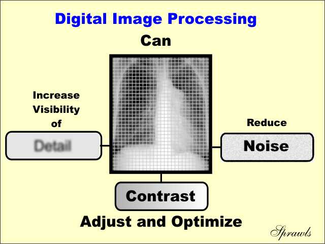
Image Enhancement:
Enhancement methods in image processing
Image enhancement is the process of adjusting digital images so that the results are more suitable for display or further image analysis. For example, you can remove noise, sharpen, or brighten an image, making it easier to identify key features.
Here are some useful examples and methods of image enhancement:
1. Filtering with morphological operators
2. Histogram equalization
3. Noise removal using a Wiener filter
4. Linear contrast adjustment
5. Median filtering
6. Unsharp mask filtering
7. Contrast-limited adaptive histogram equalization (CLAHE)
8. Decorrelation stretch
The following images illustrate a few of these examples:

Correcting nonuniform illumination with morphological operators

Enhancing grayscale images with histogram equalization.

Deblurring images using a Wiener filter
Image enhancement algorithms include deblurring, filtering, and contrast methods.
Bit plane slicing
Instead of highlighting gray level images, highlighting the contribution made to total image appearance by specific bits might be desired. Suppose that each pixel in an image is represented by 8 bits. Imagine the image is composed of 8, 1-bit planes ranging from bit plane1-0 (LSB)to bit plane 7 (MSB).
In terms of 8-bits bytes, plane 0 contains all lowest order bits in the bytes comprising the pixels in the image and plane 7 contains all high order bits.
A bit plane of a digital discrete signal (such as image or sound) is a set of bits corresponding to a given bit position in each of the binary numbers representing the signal.
For example, for 16-bit data representation there are 16 bit planes: the first bit plane contains the set of the most significant bit, and the 16th contains the least significant bit.
It is possible to see that the first bit plane gives the roughest but the most critical approximation of values of a medium, and the higher the number of the bit plane, the less is its contribution to the final stage. Thus, adding a bit plane gives a better approximation.
If a bit on the nth bit plane on an m-bit dataset is set to 1, it contributes a value of 2(m-n), otherwise it contributes nothing. Therefore, bit planes can contribute half of the value of the previous bit plane.

Spatial filtering
A spatial filter is an optical device which uses the principles of Fourier optics to alter the structure of a beam of coherent light or other electromagnetic radiation. Spatial filtering is commonly used to "clean up" the output of lasers, removing aberrations in the beam due to imperfect, dirty, or damaged optics, or due to variations in the laser gain medium itself. This can be used to produce a laser beam containing only a single transverse mode of the lasers optical resonator.
In spatial filtering, a lens is used to focus the beam. Because of diffraction, a beam that is not a perfect plane wave will not focus to a single spot, but rather will produce a pattern of light and dark regions in the focal plane. For example, an imperfect beam might form a bright spot surrounded by a series of concentric rings, as shown in the figure to the right. It can be shown that this two-dimensional pattern is the two-dimensional Fourier transform of the initial beams transverse intensity distribution. In this context, the focal plane is often called the transform plane. Light in the very center of the transform pattern corresponds to a perfect, wide plane wave. Other light corresponds to "structure" in the beam, with light further from the central spot corresponding to structure with higher spatial frequency. A pattern with very fine details will produce light very far from the transform planes central spot. In the example above, the large central spot and rings of light surrounding it are due to the structure resulting when the beam passed through a circular aperture. The spot is enlarged because the beam is limited by the aperture to a finite size, and the rings relate to the sharp edges of the beam created by the edges of the aperture. This pattern is called an Airy pattern, after its discoverer George Airy.
By altering the distribution of light in the transform plane and using another lens to reform the collimated beam, the structure of the beam can be altered. The most common way of doing this is to place an aperture in the beam that allows the desired light to pass, while blocking light that corresponds to undesired structure in the beam. In particular, a small circular aperture or "pinhole" that passes only the central bright spot can remove nearly all fine structure from the beam, producing a smooth transverse intensity profile, which may be almost a perfect gaussian beam. With good optics and a very small pinhole, one could even approximate a plane wave.
In practice, the diameter of the aperture is chosen based on the focal length of the lens, the diameter and quality of the input beam, and its wavelength (longer wavelengths require larger apertures). If the hole is too small, the beam quality is greatly improved but the power is greatly reduced. If the hole is too large, the beam quality may not be improved as much as desired.
homomorphic filtering
Homomorphic filter is sometimes used for image enhancement. It simultaneously normalizes the brightness across an image and increases contrast. Here homomorphic filtering is used to remove multiplicative noise. Illumination and reflectance are not separable, but their approximate locations in the frequency domain may be located. Since illumination and reflectance combine multiplicatively, the components are made additive by taking the logarithm of the image intensity, so that these multiplicative components of the image can be separated linearly in the frequency domain. Illumination variations can be thought of as a multiplicative noise, and can be reduced by filtering in the log domain.
Image Restoration and Denoising
refer this link for detailed information
https://fenix.tecnico.ulisboa.pt/downloadFile/3779576309408/4_%20Image_restoration.pdf
Image Degradation
Image degradation is said to occur when acertain image under goes loss of storedinformation either due to digitization orconversion (i.e algortithmic operations),decreasing visiual quality.
Image restoration
Image restoration is the operation of taking a corrupted/noisy image and estimating the clean original image. Corruption may come in many forms such as motion blur, noise, and camera misfocus.
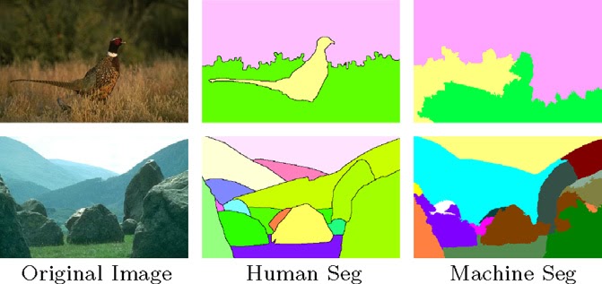
Image segmentation
In computer vision, image segmentation is the process of partitioning a digital image into multiple segments (sets of pixels, also known as superpixels). The goal of segmentation is to simplify and/or change the representation of an image into something that is more meaningful and easier to analyze. Image segmentation is typically used to locate objects and boundaries (lines, curves, etc.) in images. More precisely, image segmentation is the process of assigning a label to every pixel in an image such that pixels with the same label share certain characteristics.
The result of image segmentation is a set of segments that collectively cover the entire image, or a set of contours extracted from the image (see edge detection). Each of the pixels in a region are similar with respect to some characteristic or computed property, such as color, intensity, or texture. Adjacent regions are significantly different with respect to the same characteristic(s).When applied to a stack of images, typical in medical imaging, the resulting contours after image segmentation can be used to create 3D reconstructions with the help of interpolation algorithms like Marching cubes.
Thresholding
The simplest method of image segmentation is called the thresholding method. This method is based on a clip-level (or a threshold value) to turn a gray-scale image into a binary image. There is also a balanced histogram thresholding.
The key of this method is to select the threshold value (or values when multiple-levels are selected). Several popular methods are used in industry including the maximum entropy method, Otsus method (maximum variance), and k-means clustering.
Recently, methods have been developed for thresholding computed tomography (CT) images. The key idea is that, unlike Otsus method, the thresholds are derived from the radiographs instead of the (reconstructed) image.
Image Data Compression
The objective of image compression is to reduce irrelevance and redundancy of the image data in order to be able to store or transmit data in an efficient form.
Image compression may be lossy or lossless. Lossless compression is preferred for archival purposes and often for medical imaging, technical drawings, clip art, or comics. Lossy compression methods, especially when used at low bit rates, introduce compression artifacts. Lossy methods are especially suitable for natural images such as photographs in applications where minor (sometimes imperceptible) loss of fidelity is acceptable to achieve a substantial reduction in bit rate. The lossy compression that produces imperceptible differences may be called visually lossless.
The quality of a compression method often is measured by the Peak signal-to-noise ratio. It measures the amount of noise introduced through a lossy compression of the image, however, the subjective judgment of the viewer also is regarded as an important measure, perhaps, being the most important measure.

In computer science and information theory, data compression, source coding, or bit-rate reduction involves encoding information using fewer bits than the original representation. Compression can be either lossy or lossless. Lossless compression reduces bits by identifying and eliminating statistical redundancy. No information is lost in lossless compression. Lossy compression reduces bits by identifying unnecessary information and removing it. The process of reducing the size of a data file is popularly referred to as data compression, although its formal name is source coding (coding done at the source of the data before it is stored or transmitted).
Compression is useful because it helps reduce resource usage, such as data storage space or transmission capacity. Because compressed data must be decompressed to use, this extra processing imposes computational or other costs through decompression; this situation is far from being a free lunch. Data compression is subject to a space–time complexity trade-off. For instance, a compression scheme for video may require expensive hardware for the video to be decompressed fast enough to be viewed as it is being decompressed, and the option to decompress the video in full before watching it may be inconvenient or require additional storage. The design of data compression schemes involves trade-offs among various factors, including the degree of compression, the amount of distortion introduced (e.g., when using lossy data compression), and the computational resources required to compress and uncompress the data.