Taylor's theorem

Motivation

If a real-valued function f is differentiable at the point a then it has a linear approximation at the point a. This means that there exists a function h₁ such that

Here

is the linear approximation of f at the point a. The graph of y = P₁(x) is the tangent line to the graph of f at x = a. The error in the approximation is

Note that this goes to zero a little bit faster than x − a as x tends to a, given the limiting behavior of h₁.

If we wanted a better approximation to f, we might instead try a quadratic polynomial instead of a linear function. Instead of just matching one derivative of f at a, we can match two derivatives, thus producing a polynomial that has the same slope and concavity as f at a. The quadratic polynomial in question is

Taylor's theorem ensures that the quadratic approximation is, in a sufficiently small neighborhood of the point a, a better approximation than the linear approximation. Specifically,

Here the error in the approximation is

which, given the limiting behavior of h 2 , goes to zero faster than ( x − a ) 2 as x tends to a.

Similarly, we might get still better approximations to f if we use polynomials of higher degree, since then we can match even more derivatives with f at the selected base point.

In general, the error in approximating a function by a polynomial of degree k will go to zero a little bit faster than (x − a)^k as x tends to a. But this might not always be the case: it is also possible that increasing the degree of the approximating polynomial does not increase the quality of approximation at all even if the function f to be approximated is infinitely many times differentiable. An example of this behavior is given below, and it is related to the fact that unlike analytic functions, more general functions are not (locally) determined by the values of their derivatives at a single point.

Taylor's theorem is of asymptotic nature: it only tells us that the error R_k in an approximation by a k-th order Taylor polynomial P_k tends to zero faster than any nonzero k-th degree polynomial as x → a. It does not tell us how large the error is in any concrete neighborhood of the center of expansion, but for this purpose there are explicit formulae for the remainder term (given below) which are valid under some additional regularity assumptions on f. These enhanced versions of Taylor's theorem typically lead to uniform estimates for the approximation error in a small neighborhood of the center of expansion, but the estimates do not necessarily hold for neighborhoods which are too large, even if the function f is analytic. In that situation one may have to select several Taylor polynomials with different centers of expansion to have reliable Taylor-approximations of the original function (see animation on the right.)

There are several things we might do with the remainder term:

1. Estimate the error in using a polynomial P_k(x) of degree k to estimate f(x) on a given interval (a - r, a + r). (The interval and the degree k are fixed; we want to find the error.)
2. Find the smallest degree k for which the polynomial P_k(x) approximates f(x) to within a given error (or tolerance) on a given interval (a - r, a + r) . (The interval and the error are fixed; we want to find the degree.)
3. Find the largest interval (a - r, a + r) on which P_k(x) approximates f(x) to within a given error ("tolerance"). (The degree and the error are fixed; we want to find the interval.)

Statement of the theorem

The precise statement of the most basic version of Taylor's theorem is as follows:

The polynomial appearing in Taylor's theorem is the k-th order Taylor polynomial

of the function f at the point a. The Taylor polynomial is the unique "asymptotic best fit" polynomial in the sense that if there exists a function h_k : R → R and a k-th order polynomial p such that

then p = P_k. Taylor's theorem describes the asymptotic behavior of the remainder term

which is the approximation error when approximating f with its Taylor polynomial. Using the little-o notation the statement in Taylor's theorem reads as

Explicit formulas for the remainder

Under stronger regularity assumptions on f there are several precise formulae for the remainder term R_k of the Taylor polynomial, the most common ones being the following.

These refinements of Taylor's theorem are usually proved using the mean value theorem, whence the name. Also other similar expressions can be found. For example, if G(t) is continuous on the closed interval and differentiable with a non-vanishing derivative on the open interval between a and x, then

for some number ξ between a and x. This version covers the Lagrange and Cauchy forms of the remainder as special cases, and is proved below using Cauchy's mean value theorem.

The statement for the integral form of the remainder is more advanced than the previous ones, and requires understanding of Lebesgue integration theory for the full generality. However, it holds also in the sense of Riemann integral provided the (k + 1)th derivative of f is continuous on the closed interval [a,x].

Due to absolute continuity of f^(k) on the closed interval between a and x its derivative f^(k+1) exists as an L¹-function, and the result can be proven by a formal calculation using fundamental theorem of calculus and integration by parts.

Estimates for the remainder

It is often useful in practice to be able to estimate the remainder term appearing in the Taylor approximation, rather than having an exact formula for it. Suppose that f is (k + 1)-times continuously differentiable in an interval I containing a. Suppose that there are real constants q and Q such that

throughout I. Then the remainder term satisfies the inequality

if x > a, and a similar estimate if x < a. This is a simple consequence of the Lagrange form of the remainder. In particular, if

on an interval I = (a − r,a + r) with some r > 0 , then

for all x∈(a − r,a + r). The second inequality is called a uniform estimate, because it holds uniformly for all x on the interval (a − r,a + r).

Example

Suppose that we wish to approximate the function f(x) = e^x on the interval [−1,1] while ensuring that the error in the approximation is no more than 10⁻⁵. In this example we pretend that we only know the following properties of the exponential function:

From these properties it follows that f^(k)(x) = e^x for all k, and in particular, f^(k)(0) = 1. Hence the k-th order Taylor polynomial of f at 0 and its remainder term in the Lagrange form are given by

where ξ is some number between 0 and x. Since e^x is increasing by (*), we can simply use e^x ≤ 1 for x ∈ [−1, 0] to estimate the remainder on the subinterval [−1, 0]. To obtain an upper bound for the remainder on [0,1], we use the property e^ξ<e^x for 0<ξ<x to estimate

using the second order Taylor expansion. Then we solve for e^x to deduce that

simply by maximizing the numerator and minimizing the denominator. Combining these estimates for e^x we see that

so the required precision is certainly reached, when

(See factorial or compute by hand the values 9!=362 880 and 10!=3 628 800.) As a conclusion, Taylor's theorem leads to the approximation

For instance, this approximation provides a decimal expression e ≈ 2.71828, correct up to five decimal places.

Taylor expansions of real analytic functions

Let I ⊂ R be an open interval. By definition, a function f : I → R is real analytic if it is locally defined by a convergent power series. This means that for every a ∈ I there exists some r > 0 and a sequence of coefficients c_k ∈ R such that (a − r, a + r) ⊂ I and

In general, the radius of convergence of a power series can be computed from the Cauchy–Hadamard formula

This result is based on comparison with a geometric series, and the same method shows that if the power series based on a converges for some b ∈ R, it must converge uniformly on the closed interval [a − r_b, a + r_b], where r_b = |b − a|. Here only the convergence of the power series is considered, and it might well be that (a − R,a + R) extends beyond the domain I of f.

The Taylor polynomials of the real analytic function f at a are simply the finite truncations

of its locally defining power series, and the corresponding remainder terms are locally given by the analytic functions

Here the functions

are also analytic, since their defining power series have the same radius of convergence as the original series. Assuming that [a − r, a + r] ⊂ I and r < R, all these series converge uniformly on (a − r, a + r). Naturally, in the case of analytic functions one can estimate the remainder term R_k(x) by the tail of the sequence of the derivatives f′(a) at the center of the expansion, but using complex analysis also another possibility arises, which is described below.

Taylor's theorem and convergence of Taylor series

The Taylor series of f will converge in some interval, given that all its derivatives are bounded over it and do not grow too fast as k goes to infinity. (However, it is not always the case that the Taylor series of f, if it converges, will in fact converge to f, as explained below; f is then said to be non-analytic.)

One might think of the Taylor series

of an infinitely many times differentiable function f : R → R as its "infinite order Taylor polynomial" at a. Now the estimates for the remainder imply that if, for any r, the derivatives of f are known to be bounded over (a − r,a + r), then for any order k and for any r > 0 there exists a constant M_k,r > 0 such that

for every x ∈ (a − r,a + r). Sometimes the constants M_k,r can be chosen in such way that M_k,r is bounded above, for fixed r and all but finitely many k. Then the Taylor series of f converges uniformly to some analytic function

(One also gets convergence even if M_k,r is not bounded above as long as it grows slowly enough.)

However, even though T_f is always analytic, the case may be that f is not. That is to say, it may well be that an infinitely many times differentiable function f has a Taylor series at a which converges on some open neighborhood of a, but the limit function T_f is different from f. An important example of this phenomenon is provided by

Using the chain rule one can show by mathematical induction that for any order k,

for some polynomial p_k of degree 2(k − 1). The function e − 1 x 2 tends to zero faster than any polynomial as x → 0, so f is infinitely many times differentiable and f^(k)(0) = 0 for every positive integer k. Now the estimates for the remainder for the Taylor polynomials show that the Taylor series of f converges uniformly to the zero function on the whole real axis. Nothing is wrong in here:

Taylor's theorem in complex analysis

Taylor's theorem generalizes to functions f : C → C which are complex differentiable in an open subset U ⊂ C of the complex plane. However, its usefulness is dwarfed by other general theorems in complex analysis. Namely, stronger versions of related results can be deduced for complex differentiable functions f : U → C using Cauchy's integral formula as follows.

Let r > 0 such that the closed disk B(z, r) ∪ S(z, r) is contained in U. Then Cauchy's integral formula with a positive parametrization γ(t)=z + re^it of the circle S(z, r) with t ∈ [0, 2π] gives

Here all the integrands are continuous on the circle S(z, r), which justifies differentiation under the integral sign. In particular, if f is once complex differentiable on the open set U, then it is actually infinitely many times complex differentiable on U. One also obtains the Cauchy's estimates

for any z ∈ U and r > 0 such that B(z, r) ∪ S(c, r) ⊂ U. These estimates imply that the complex Taylor series

of f converges uniformly on any open disk B(c, r) ⊂ U with S(c, r) ⊂ U into some function T_f. Furthermore, using the contour integral formulae for the derivatives f^(k)(c),

so any complex differentiable function f in an open set U ⊂ C is in fact complex analytic. All that is said for real analytic functions here holds also for complex analytic functions with the open interval I replaced by an open subset U ∈ C and a-centered intervals (a − r, a + r) replaced by c-centered disks B(c, r). In particular, the Taylor expansion holds in the form

where the remainder term R_k is complex analytic. Methods of complex analysis provide some powerful results regarding Taylor expansions. For example, using Cauchy's integral formula for any positively oriented Jordan curve γ which parametrizes the boundary ∂W ⊂ U of a region W ⊂ U, one obtains expressions for the derivatives f^(j)(c) as above, and modifying slightly the computation for T_f(z) = f(z), one arrives at the exact formula

The important feature here is that the quality of the approximation by a Taylor polynomial on the region W ⊂ U is dominated by the values of the function f itself on the boundary ∂W ⊂ U. Similarly, applying Cauchy's estimates to the series expression for the remainder, one obtains the uniform estimates

Example

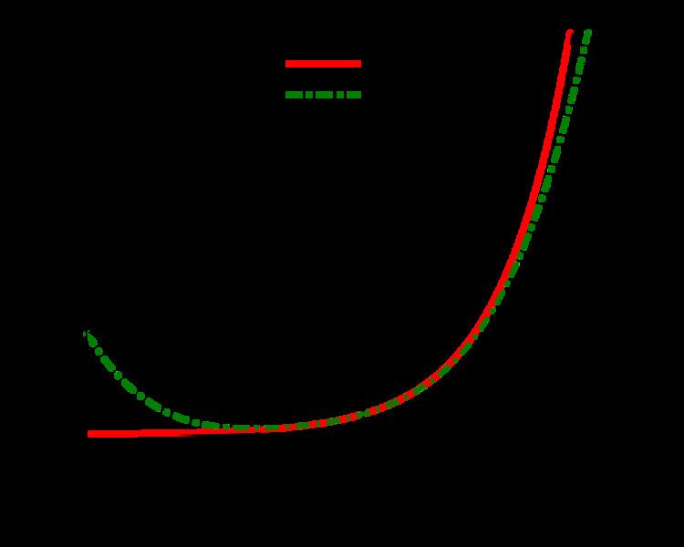
The function

is real analytic, that is, locally determined by its Taylor series. This function was plotted above to illustrate the fact that some elementary functions cannot be approximated by Taylor polynomials in neighborhoods of the center of expansion which are too large. This kind of behavior is easily understood in the framework of complex analysis. Namely, the function f extends into a meromorphic function

on the compactified complex plane. It has simple poles at z = i and z = −i, and it is analytic elsewhere. Now its Taylor series centered at z₀ converges on any disc B(z₀, r) with r < |z − z₀|, where the same Taylor series converges at z ∈ C. Therefore, Taylor series of f centered at 0 converges on B(0, 1) and it does not converge for any z ∈ C with |z| > 1 due to the poles at i and −i. For the same reason the Taylor series of f centered at 1 converges on B(1, √2) and does not converge for any z ∈ C with |z − 1| > √2.

Higher-order differentiability

A function f: Rⁿ → R is differentiable at a ∈ Rⁿ if and only if there exists a linear functional L : Rⁿ → R and a function h : Rⁿ → R such that

If this is the case, then L = df(a) is the (uniquely defined) differential of f at the point a. Furthermore, then the partial derivatives of f exist at a and the differential of f at a is given by

Introduce the multi-index notation

for α ∈ Nⁿ and x ∈ Rⁿ. If all the k-th order partial derivatives of f : Rⁿ → R are continuous at a ∈ Rⁿ, then by Clairaut's theorem, one can change the order of mixed derivatives at a, so the notation

for the higher order partial derivatives is justified in this situation. The same is true if all the (k − 1)-th order partial derivatives of f exist in some neighborhood of a and are differentiable at a. Then we say that f is k times differentiable at the point a .

Taylor's theorem for multivariate functions

If the function f : Rⁿ → R is k + 1 times continuously differentiable in the closed ball B, then one can derive an exact formula for the remainder in terms of (k+1)-th order partial derivatives of f in this neighborhood. Namely,

In this case, due to the continuity of (k+1)-th order partial derivatives in the compact set B, one immediately obtains the uniform estimates

Example in two dimensions

For example, the third-order Taylor polynomial of a smooth function f: R² → R is, denoting x − a = v,

Proof for Taylor's theorem in one real variable

Let

where, as in the statement of Taylor's theorem,

It is sufficient to show that

The proof here is based on repeated application of L'Hôpital's rule. Note that, for each j = 0,1,...,k−1, f ( j ) ( a ) = P ( j ) ( a ) . Hence each of the first k−1 derivatives of the numerator in h k ( x ) vanishes at x = a , and the same is true of the denominator. Also, since the condition that the function f be k times differentiable at a point requires differentiability up to order k−1 in a neighborhood of said point (this is true, because differentiability requires a function to be defined in a whole neighborhood of a point), the numerator and its k-2 derivatives are differentiable in a neighborhood of a. Clearly, the denominator also satisfies said condition, and additionally, doesn't vanish unless x=a, therefore all conditions necessary for L'Hopital's rule are fulfilled, and its use is justified. So

where the second to last equality follows by the definition of the derivative at x = a.

Derivation for the mean value forms of the remainder

Let G be any real-valued function, continuous on the closed interval between a and x and differentiable with a non-vanishing derivative on the open interval between a and x, and define

Then, by Cauchy's mean value theorem,

for some ξ on the open interval between a and x. Note that here the numerator F(x) − F(a) = R_k(x) is exactly the remainder of the Taylor polynomial for f(x). Compute

plug it into (*) and rearrange terms to find that

This is the form of the remainder term mentioned after the actual statement of Taylor's theorem with remainder in the mean value form. The Lagrange form of the remainder is found by choosing   G ( t ) = ( x − t ) k + 1   and the Cauchy form by choosing   G ( t ) = t − a .

Remark. Using this method one can also recover the integral form of the remainder by choosing

but the requirements for f needed for the use of mean value theorem are too strong, if one aims to prove the claim in the case that f^(k) is only absolutely continuous. However, if one uses Riemann integral instead of Lebesgue integral, the assumptions cannot be weakened.

Derivation for the integral form of the remainder

Due to absolute continuity of f^(k) on the closed interval between a and x its derivative f^(k+1) exists as an L¹-function, and we can use fundamental theorem of calculus and integration by parts. This same proof applies for the Riemann integral assuming that f^(k) is continuous on the closed interval and differentiable on the open interval between a and x, and this leads to the same result than using the mean value theorem.

The fundamental theorem of calculus states that

Now we can integrate by parts and use the fundamental theorem of calculus again to see that

which is exactly Taylor's theorem with remainder in the integral form in the case k=1. The general statement is proved using induction. Suppose that

Integrating the remainder term by parts we arrive at

Substituting this into the formula in (*) shows that if it holds for the value k, it must also hold for the value k + 1. Therefore, since it holds for k = 1, it must hold for every positive integer k.

Derivation for the remainder of multivariate Taylor polynomials

We prove the special case, where f : Rⁿ → R has continuous partial derivatives up to the order k+1 in some closed ball B with center a. The strategy of the proof is to apply the one-variable case of Taylor's theorem to the restriction of f to the line segment adjoining x and a. Parametrize the line segment between a and x by u(t) = a + t(x − a). We apply the one-variable version of Taylor's theorem to the function g(t) = f(u(t)):

Applying the chain rule for several variables gives

where ( j α ) is the multinomial coefficient. Since 1 j ! ( j α ) = 1 α ! , we get