Simpson's rule

Derivation

Simpson's rule can be derived in various ways.

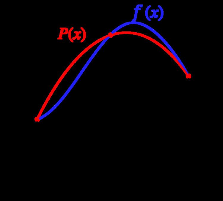
Quadratic interpolation

One derivation replaces the integrand f ( x ) by the quadratic polynomial (i.e. parabola) P ( x ) which takes the same values as f ( x ) at the end points a and b and the midpoint m = (a + b) / 2. One can use Lagrange polynomial interpolation to find an expression for this polynomial,

An easy (albeit tedious) integration by substitution shows that

This calculation can be carried out more easily if one first observes that (by scaling) there is no loss of generality in assuming that a = − 1 and b = 1 .

Averaging the midpoint and the trapezoidal rules

Another derivation constructs Simpson's rule from two simpler approximations: the midpoint rule

and the trapezoidal rule

The errors in these approximations are

respectively, where O ( ( b − a ) 4 ) denotes a term asymptotically proportional to ( b − a ) 4 . The two O ( ( b − a ) 4 ) terms are not equal; see Big O notation for more details. It follows from the above formulas for the errors of the midpoint and trapezoidal rule that the leading error term vanishes if we take the weighted average

This weighted average is exactly Simpson's rule.

Using another approximation (for example, the trapezoidal rule with twice as many points), it is possible to take a suitable weighted average and eliminate another error term. This is Romberg's method.

Undetermined coefficients

The third derivation starts from the ansatz

The coefficients α, β and γ can be fixed by requiring that this approximation be exact for all quadratic polynomials. This yields Simpson's rule.

Error

The error in approximating an integral by Simpson's rule is

where ξ is some number between a and b .

The error is asymptotically proportional to ( b − a ) 5 . However, the above derivations suggest an error proportional to ( b − a ) 4 . Simpson's rule gains an extra order because the points at which the integrand is evaluated are distributed symmetrically in the interval [a, b].

Since the error term is proportional to the fourth derivative of f at ξ , this shows that Simpson's rule provides exact results for any polynomial f of degree three or less, since the fourth derivative of such a polynomial is zero at all points.

Composite Simpson's rule

If the interval of integration [ a , b ] is in some sense "small", then Simpson's rule will provide an adequate approximation to the exact integral. By small, what we really mean is that the function being integrated is relatively smooth over the interval [ a , b ] . For such a function, a smooth quadratic interpolant like the one used in Simpson's rule will give good results.

However, it is often the case that the function we are trying to integrate is not smooth over the interval. Typically, this means that either the function is highly oscillatory, or it lacks derivatives at certain points. In these cases, Simpson's rule may give very poor results. One common way of handling this problem is by breaking up the interval [ a , b ] into a number of small subintervals. Simpson's rule is then applied to each subinterval, with the results being summed to produce an approximation for the integral over the entire interval. This sort of approach is termed the composite Simpson's rule.

Suppose that the interval [ a , b ] is split up into n subintervals, with n an even number. Then, the composite Simpson's rule is given by

where x j = a + j h for j = 0 , 1 , . . . , n − 1 , n with h = ( b − a ) / n ; in particular, x 0 = a and x n = b . This composite rule with n = 2 corresponds with the regular Simpson's Rule of the preceding section. The above formula can also be written as

The error committed by the composite Simpson's rule is bounded (in absolute value) by

where h is the "step length", given by h = ( b − a ) / n .

This formulation splits the interval [ a , b ] in subintervals of equal length. In practice, it is often advantageous to use subintervals of different lengths, and concentrate the efforts on the places where the integrand is less well-behaved. This leads to the adaptive Simpson's method.

Alternative extended Simpson's rule

This is another formulation of a composite Simpson's rule: instead of applying Simpson's rule to disjoint segments of the integral to be approximated, Simpson's rule is applied to overlapping segments, yielding:

The formula above is obtained by combining the original composite Simpson's rule with the one consisting in using Simpson's 3/8 rule in the extreme subintervals and the standard 3-point rule in the remaining subintervals. The result is then obtained by taking the mean of the two formulas.

Simpson's 3/8 rule

Simpson's 3/8 rule is another method for numerical integration proposed by Thomas Simpson. It is based upon a cubic interpolation rather than a quadratic interpolation. Simpson's 3/8 rule is as follows:

where b - a = 3h. The error of this method is:

where ξ is some number between a and b . Thus, the 3/8 rule is about twice as accurate as the standard method, but it uses one more function value. A composite 3/8 rule also exists, similarly as above.

A further generalization of this concept for interpolation with arbitrary degree polynomials are the Newton–Cotes formulas.

Simpson's 3/8 rule (for n intervals)

Defining,

we have

Note, we can only use this if n is a multiple of three.

A simplified version of Simpson's rules is used in naval architecture. The 3/8th rule is also called Simpson's Second Rule.

Sample implementation

An implementation of the composite Simpson's rule in Python:

Note that this function is available in SciPy as scipy.integrate.simps.