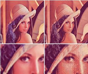
Ordered dithering

Ordered dithering is an image dithering algorithm. It is commonly used by programs that need to provide continuous image of higher colors on a display of less color depth. For example, Microsoft Windows uses it in 16-color graphics modes. It is easily distinguished by its noticeable crosshatch patterns.

The algorithm achieves dithering by applying a threshold map M on the pixels displayed, causing some of the pixels to be rendered at a different color, depending on how far in between the color is of available color entries.

Different sizes of threshold maps exist:

The map may be rotated or mirrored without affecting the effectiveness of the algorithm. This threshold map (for sides with length as power of two) is also known as an index matrix or Bayer matrix.

Arbitrary size threshold maps can be devised with a simple rule: First fill each slot with a successive integers. Then reorder them such that the average distance between two successive numbers in the map is as large as possible, ensuring that the table "wraps" around at edges. For threshold maps whose dimensions are a power of two, the map can be generated recursively via:

M 2 n = 1 4 × [ 4 × M n 4 × M n + 2 4 × M n + 3 4 × M n + 1 ]

The recursive expression can be calculated explicitly using only bit arithmetic:

M(i, j) = bit_reverse(bit_interleave(bitwise_xor(x, y), x)) / n ^ 2

The algorithm renders the image normally, but for each pixel, it adds a value from the threshold map, causing the pixel's value to be quantized one step higher if it exceeds the threshold. For example, in monochrome rendering, if the value of the pixel (scaled into the 0-9 range if using a 3x3 matrix) is less than the number in the corresponding cell of the matrix, plot that pixel black, otherwise, plot it white.

The algorithm performs the following transformation on each color c of every pixel:

c ′ = n e a r e s t _ p a l e t t e _ c o l o r ( c + r × ( M ( x mod n , y mod n ) − 1 2 ) )

where M(i, j) is the threshold map on the i-th row and j-th column, c′ is the transformed color, and r is the amount of spread in color space. Assuming an RGB palette with N³ evenly chosen colors where each color coordinate is represented by an octet, one would typically choose:

r ≈ 256 N

The values read from the threshold map should scale into the same range as is the minimal difference between distinct colors in the target palette.

Because the algorithm operates on single pixels and has no conditional statements, it is very fast and suitable for real-time transformations. Additionally, because the location of the dithering patterns stays always the same relative to the display frame, it is less prone to jitter than error-diffusion methods, making it suitable for animations. Because the patterns are more repetitive than error-diffusion method, an image with ordered dithering compresses better. Ordered dithering is more suitable for line-art graphics as it will result in straighter lines and fewer anomalies.

The size of the map selected should be equal to or larger than the ratio of source colors to target colors. For example, when quantizing a 24bpp image to 15bpp (256 colors per channel to 32 colors per channel), the smallest map one would choose would be 4x2, for the ratio of 8 (256:32). This allows expressing each distinct tone of the input with different dithering patterns.