Mathematical Modeling of Mercury Thermometer

A mathematical model is use to study the behavior of a system as it evolves over time.Mathematical model basically takes the form of a set of assumptions related to operation of the system.These assumptions are expressed in form of mathematical or logical relationships between the entities of system.

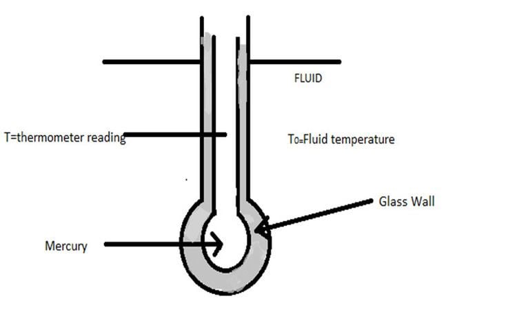
Let us consider an mercury thermometer which is located in a flowing stream of fluid for which temperature T0 varies with time.We have to calculate the response or the time variation of the thermometer reading T for a particular change in T0.

Following assumptions are made for the analysis:

1. The resistance to heat transfer offered by glass and mercury is negligible.So all the resistance to heat transfer is present in the film surrounding the bulb.

2. At any instant mercury assumes a uniform temperature throughout.And all the thermal capacity is in the mercury.

The above 2 assumptions are known as lumping of parameters because all the resistance is “lumped” into one location and all the capacitance into another.Thus it is a lumped model of mercury thermometer.

3. There is no expansion or contraction in the glass wall

which contains mercury during the transient response.

(Hence mercury reading will not rise or fall due to change in volume of glass wall).

4.Initially thermometer is assumed to be at steady state at t=0.

Diagram:

Energy balance:

On applying the unsteady-state energy balance

(Input rate) -(output rate)=(Rate of accumulation)

We get ,

m c d T d t = h A ( T 0 − T ) (1)

Ԏ d T d t + T = T 0 (2)

where Ԏ = m c / h A

m = mass of mercury in bulb

c = heat capacity of mercury

A = surface area of bulb for heat transfer

t = time

h =film coefficient of heat transfer

Ԏ = time constant of the system

At steady state,

T s = T 0 s (3) for t≤ 0

Subtracting (3) from (2) we get

Ԏ d ( T − T s ) d t + ( T − T s ) = ( T 0 − T 0 s ) (4)

Let Y = T − T s & X = T o − T o s

where Y, X are known as deviation variables.

Therefore equation (4) become

Ԏ d Y d T + Y = X (5)

Taking Laplace transform on equation (5),we get

Ԏ s Y ( s ) + Y ( s ) = X ( s ) (6)

Y ( s ) [ 1 + Ԏ s ] = X ( s ) (7)

G ( s ) = Y ( s ) / X ( s ) = 1 / ( 1 + Ԏ s ) = O U T P U T / I N P U T

G(s) is the transfer function.

X(s) = Transform of forcing function or input, in deviation form

Y(s) = Transform of response or output, in deviation form.

Transfer function is the ratio of the Laplace transform of the deviation in thermometer reading (output) to the Laplace transform of the deviation in the surrounding temperature (input).

We can find the response of the system or output by giving various types of inputs like step input, impulse input, sinusoidal input,etc.