Interference (wave propagation) - Alchetron, the free social encyclopedia

In physics, interference is a phenomenon in which two waves superpose to form a resultant wave of greater, lower, or the same amplitude. Interference usually refers to the interaction of waves that are correlated or coherent with each other, either because they come from the same source or because they have the same or nearly the same frequency. Interference effects can be observed with all types of waves, for example, light, radio, acoustic, surface water waves or matter waves.

Mechanisms

The principle of superposition of waves states that when two or more propagating waves of same type are incident on the same point, the resultant amplitude at that point is equal to the vector sum of the amplitudes of the individual waves. If a crest of a wave meets a crest of another wave of the same frequency at the same point, then the amplitude is the sum of the individual amplitudes—this is constructive interference. If a crest of one wave meets a trough of another wave, then the amplitude is equal to the difference in the individual amplitudes—this is known as destructive interference.

Constructive interference occurs when the phase difference between the waves is an even multiple of π (180°) (a multiple of 2π, 360°), whereas destructive interference occurs when the difference is an odd multiple of π. If the difference between the phases is intermediate between these two extremes, then the magnitude of the displacement of the summed waves lies between the minimum and maximum values.

Consider, for example, what happens when two identical stones are dropped into a still pool of water at different locations. Each stone generates a circular wave propagating outwards from the point where the stone was dropped. When the two waves overlap, the net displacement at a particular point is the sum of the displacements of the individual waves. At some points, these will be in phase, and will produce a maximum displacement. In other places, the waves will be in anti-phase, and there will be no net displacement at these points. Thus, parts of the surface will be stationary—these are seen in the figure above and to the right as stationary blue-green lines radiating from the centre.

Interference of light is a common phenomenon that can be explained classically by the superposition of waves theory however a deeper understanding of light interference requires knowledge of the quantum wave propagation of light which resolves further experimental observations, see QED: The Strange Theory of Light and Matter. Prime examples of light interference are the famous Double-slit experiment ( see Copenhagen interpretation), laser speckle, optical thin layers and films and interferometers. An example is the double slit experiment, classically light interferes and the energy of photons is lost, however with wave propagation the observed bright and dark areas are a result of the paths available for the photons to travel. Dark areas in the double slit are not available to the photons and bright areas are allowed paths. Laser speckle and a Michelson interferometer are examples where an observer truly observes light of differing phases, the electrons in the photo sensitive areas of the eye do not perceive photons that are out of phase with each other due to a net zero superposition of the E vector of the photons, these photons merely continue deeper into the eye tissues where they are absorbed. Thin films also behave in a quantum manner. Traditionally the classical model is taught as a basis for understanding optical interference based the Huygens–Fresnel principle and it was not until discussions in the 1920s Solvay Conference that de Broglie first proposed unique wave properties of light, Feynman made further significant contributions in the 1940s/50s and experiments continue today.

Derivation

The above can be demonstrated in one dimension by deriving the formula for the sum of two waves. The equation for the amplitude of a sinusoidal wave traveling to the right along the x-axis is

W 1 ( x , t ) = A cos ⁡ ( k x − ω t )

where A is the peak amplitude, k = 2 π / λ is the wavenumber and ω = 2 π f is the angular frequency of the wave. Suppose a second wave of the same frequency and amplitude but with a different phase is also traveling to the right

W 2 ( x , t ) = A cos ⁡ ( k x − ω t + ϕ )

where ϕ is the phase difference between the waves in radians. The two waves will superpose and add: the sum of the two waves is

W 1 + W 2 = A [ cos ⁡ ( k x − ω t ) + cos ⁡ ( k x − ω t + ϕ ) ]

Using the trigonometric identity for the sum of two cosines: cos ⁡ a + cos ⁡ b = 2 cos ⁡ ( a + b 2 ) cos ⁡ ( a − b 2 ) , this can be written

W 1 + W 2 = 2 A cos ⁡ ( k x − ω t + ϕ 2 ) cos ⁡ ( ϕ 2 )

This represents a wave at the original frequency, traveling to the right like the components, whose amplitude is proportional to the cosine of ϕ / 2 .

Constructive interference: If the phase difference is an even multiple of pi: ϕ = . . . − 4 π , − 2 π , 0 , 2 π , 4 π , . . . then | cos ⁡ ϕ / 2 | = 1 , so the sum of the two waves is a wave with twice the amplitude

Destructive interference: If the phase difference is an odd multiple of pi: ϕ = . . . − 3 π , − π , π , 3 π , 5 π , . . . then cos ⁡ ϕ / 2 = 0 , so the sum of the two waves is zero

Between two plane waves

A simple form of interference pattern is obtained if two plane waves of the same frequency intersect at an angle. Interference is essentially an energy redistribution process. The energy which is lost at the destructive interference is regained at the constructive interference. One wave is travelling horizontally, and the other is travelling downwards at an angle θ to the first wave. Assuming that the two waves are in phase at the point B, then the relative phase changes along the x-axis. The phase difference at the point A is given by

Δ φ = 2 π d λ = 2 π x sin ⁡ θ λ

It can be seen that the two waves are in phase when

x sin ⁡ θ λ = 0 , ± 1 , ± 2 , . . . ,

and are half a cycle out of phase when

x sin ⁡ θ λ = ± 1 2 , ± 3 2 , . . .

Constructive interference occurs when the waves are in phase, and destructive interference when they are half a cycle out of phase. Thus, an interference fringe pattern is produced, where the separation of the maxima is

d f = λ sin ⁡ θ

and d_f is known as the fringe spacing. The fringe spacing increases with increase in wavelength, and with decreasing angle θ.

The fringes are observed wherever the two waves overlap and the fringe spacing is uniform throughout.

Between two spherical waves

A point source produces a spherical wave. If the light from two point sources overlaps, the interference pattern maps out the way in which the phase difference between the two waves varies in space. This depends on the wavelength and on the separation of the point sources. The figure to the right shows interference between two spherical waves. The wavelength increases from top to bottom, and the distance between the sources increases from left to right.

When the plane of observation is far enough away, the fringe pattern will be a series of almost straight lines, since the waves will then be almost planar.

Multiple beams

Interference occurs when several waves are added together provided that the phase differences between them remain constant over the observation time.

It is sometimes desirable for several waves of the same frequency and amplitude to sum to zero (that is, interfere destructively, cancel). This is the principle behind, for example, 3-phase power and the diffraction grating. In both of these cases, the result is achieved by uniform spacing of the phases.

It is easy to see that a set of waves will cancel if they have the same amplitude and their phases are spaced equally in angle. Using phasors, each wave can be represented as A e i φ n for N waves from n = 0 to n = N − 1 , where

φ n − φ n − 1 = 2 π N .

To show that

∑ n = 0 N − 1 A e i φ n = 0

one merely assumes the converse, then multiplies both sides by e i 2 π N

The Fabry–Pérot interferometer uses interference between multiple reflections.

A diffraction grating can be considered to be a multiple-beam interferometer, since the peaks which it produces are generated by interference between the light transmitted by each of the elements in the grating; see interference vs. diffraction for further discussion.

Optical interference

Because the frequency of light waves (~10¹⁴ Hz) is too high to be detected by currently available detectors, it is possible to observe only the intensity of an optical interference pattern. The intensity of the light at a given point is proportional to the square of the average amplitude of the wave. This can be expressed mathematically as follows. The displacement of the two waves at a point r is:

U 1 ( r , t ) = A 1 ( r ) e i [ φ 1 ( r ) − ω t ] U 2 ( r , t ) = A 2 ( r ) e i [ φ 2 ( r ) − ω t ]

where A represents the magnitude of the displacement, φ represents the phase and ω represents the angular frequency.

The displacement of the summed waves is

U ( r , t ) = A 1 ( r ) e i [ φ 1 ( r ) − ω t ] + A 2 ( r ) e i [ φ 2 ( r ) − ω t ]

The intensity of the light at r is given by

I ( r ) = ∫ U ( r , t ) U ∗ ( r , t ) d t ∝ A 1 2 ( r ) + A 2 2 ( r ) + 2 A 1 ( r ) A 2 ( r ) cos ⁡ [ φ 1 ( r ) − φ 2 ( r ) ]

This can be expressed in terms of the intensities of the individual waves as

I ( r ) = I 1 ( r ) + I 2 ( r ) + 2 I 1 ( r ) I 2 ( r ) cos ⁡ [ φ 1 ( r ) − φ 2 ( r ) ]

Thus, the interference pattern maps out the difference in phase between the two waves, with maxima occurring when the phase difference is a multiple of 2π. If the two beams are of equal intensity, the maxima are four times as bright as the individual beams, and the minima have zero intensity.

The two waves must have the same polarization to give rise to interference fringes since it is not possible for waves of different polarizations to cancel one another out or add together. Instead, when waves of different polarization are added together, they give rise to a wave of a different polarization state.

Light source requirements

The discussion above assumes that the waves which interfere with one another are monochromatic, i.e. have a single frequency—this requires that they are infinite in time. This is not, however, either practical or necessary. Two identical waves of finite duration whose frequency is fixed over that period will give rise to an interference pattern while they overlap. Two identical waves which consist of a narrow spectrum of frequency waves of finite duration, will give a series of fringe patterns of slightly differing spacings, and provided the spread of spacings is significantly less than the average fringe spacing, a fringe pattern will again be observed during the time when the two waves overlap.

Conventional light sources emit waves of differing frequencies and at different times from different points in the source. If the light is split into two waves and then re-combined, each individual light wave may generate an interference pattern with its other half, but the individual fringe patterns generated will have different phases and spacings, and normally no overall fringe pattern will be observable. However, single-element light sources, such as sodium- or mercury-vapor lamps have emission lines with quite narrow frequency spectra. When these are spatially and colour filtered, and then split into two waves, they can be superimposed to generate interference fringes. All interferometry prior to the invention of the laser was done using such sources and had a wide range of successful applications.

A laser beam generally approximates much more closely to a monochromatic source, and it is much more straightforward to generate interference fringes using a laser. The ease with which interference fringes can be observed with a laser beam can sometimes cause problems in that stray reflections may give spurious interference fringes which can result in errors.

Normally, a single laser beam is used in interferometry, though interference has been observed using two independent lasers whose frequencies were sufficiently matched to satisfy the phase requirements.

It is also possible to observe interference fringes using white light. A white light fringe pattern can be considered to be made up of a 'spectrum' of fringe patterns each of slightly different spacing. If all the fringe patterns are in phase in the centre, then the fringes will increase in size as the wavelength decreases and the summed intensity will show three to four fringes of varying colour. Young describes this very elegantly in his discussion of two slit interference. Some fine examples of white light fringes can be seen here. Since white light fringes are obtained only when the two waves have travelled equal distances from the light source, they can be very useful in interferometry, as they allow the zero path difference fringe to be identified.

Optical arrangements

To generate interference fringes, light from the source has to be divided into two waves which have then to be re-combined. Traditionally, interferometers have been classified as either amplitude-division or wavefront-division systems.

In an amplitude-division system, a beam splitter is used to divide the light into two beams travelling in different directions, which are then superimposed to produce the interference pattern. The Michelson interferometer and the Mach-Zehnder interferometer are examples of amplitude-division systems.

In wavefront-division systems, the wave is divided in space—examples are Young's double slit interferometer and Lloyd's mirror.

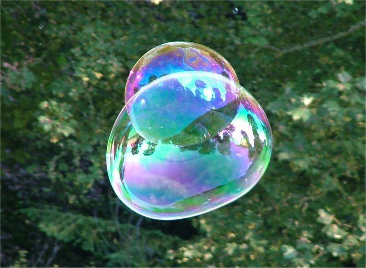
Interference can also be seen in everyday phenomena such as iridescence and structural coloration. For example, the colours seen in a soap bubble arise from interference of light reflecting off the front and back surfaces of the thin soap film. Depending on the thickness of the film, different colours interfere constructively and destructively.

Optical interferometry

Interferometry has played an important role in the advancement of physics, and also has a wide range of applications in physical and engineering measurement.

Thomas Young's double slit interferometer in 1803 demonstrated interference fringes when two small holes were illuminated by light from another small hole which was illuminated by sunlight. Young was able to estimate the wavelength of different colours in the spectrum from the spacing of the fringes. The experiment played a major role in the general acceptance of the wave theory of light. In quantum mechanics, this experiment is considered to demonstrate the inseparability of the wave and particle natures of light and other quantum particles (wave–particle duality). Richard Feynman was fond of saying that all of quantum mechanics can be gleaned from carefully thinking through the implications of this single experiment.

The results of the Michelson–Morley experiment are generally considered to be the first strong evidence against the theory of a luminiferous aether and in favor of special relativity.

Interferometry has been used in defining and calibrating length standards. When the metre was defined as the distance between two marks on a platinum-iridium bar, Michelson and Benoît used interferometry to measure the wavelength of the red cadmium line in the new standard, and also showed that it could be used as a length standard. Sixty years later, in 1960, the metre in the new SI system was defined to be equal to 1,650,763.73 wavelengths of the orange-red emission line in the electromagnetic spectrum of the krypton-86 atom in a vacuum. This definition was replaced in 1983 by defining the metre as the distance travelled by light in vacuum during a specific time interval. Interferometry is still fundamental in establishing the calibration chain in length measurement.

Interferometry is used in the calibration of slip gauges (called gauge blocks in the US) and in coordinate-measuring machines. It is also used in the testing of optical components.

Radio interferometry

In 1946, a technique called astronomical interferometry was developed. Astronomical radio interferometers usually consist either of arrays of parabolic dishes or two-dimensional arrays of omni-directional antennas. All of the telescopes in the array are widely separated and are usually connected together using coaxial cable, waveguide, optical fiber, or other type of transmission line. Interferometry increases the total signal collected, but its primary purpose is to vastly increase the resolution through a process called Aperture synthesis. This technique works by superposing (interfering) the signal waves from the different telescopes on the principle that waves that coincide with the same phase will add to each other while two waves that have opposite phases will cancel each other out. This creates a combined telescope that is equivalent in resolution (though not in sensitivity) to a single antenna whose diameter is equal to the spacing of the antennas furthest apart in the array.

Acoustic interferometry

An acoustic interferometer is an instrument for measuring the physical characteristics of sound wave in a gas or liquid. It may be used to measure velocity, wavelength, absorption, or impedance. A vibrating crystal creates the ultrasonic waves that are radiated into the medium. The waves strike a reflector placed parallel to the crystal. The waves are then reflected back to the source and measured.

Quantum interference

If a system is in state ψ , its wavefunction is described in Dirac or bra–ket notation as:

| ψ ⟩ = ∑ i | i ⟩ ⟨ i | ψ ⟩ = ∑ i | i ⟩ ψ i

where the | i ⟩ s specify the different quantum "alternatives" available (technically, they form an eigenvector basis) and the ψ i are the probability amplitude coefficients, which are complex numbers.

The probability of observing the system making a transition or quantum leap from state ψ to a new state φ is the square of the modulus of the scalar or inner product of the two states:

prob ⁡ ( ψ ⇒ φ ) = | ⟨ ψ | φ ⟩ | 2 = | ∑ i ψ i ∗ φ i | 2 = ∑ i j ψ i ∗ ψ j φ j ∗ φ i = ∑ i | ψ i | 2 | φ i | 2 + ∑ i j ; i ≠ j ψ i ∗ ψ j φ j ∗ φ i

where ψ i = ⟨ i | ψ ⟩ (as defined above) and similarly φ i = ⟨ i | φ ⟩ are the coefficients of the final state of the system. * is the complex conjugate so that ψ i ∗ = ⟨ ψ | i ⟩ , etc.

Now let's consider the situation classically and imagine that the system transited from | ψ ⟩ to | φ ⟩ via an intermediate state | i ⟩ . Then we would classically expect the probability of the two-step transition to be the sum of all the possible intermediate steps. So we would have

prob ⁡ ( ψ ⇒ φ ) = ∑ i prob ⁡ ( ψ ⇒ i ⇒ φ ) = ∑ i | ⟨ ψ | i ⟩ | 2 | ⟨ i | φ ⟩ | 2 = ∑ i | ψ i | 2 | φ i | 2 ,

The classical and quantum derivations for the transition probability differ by the presence, in the quantum case, of the extra terms ∑ i j ; i ≠ j ψ i ∗ ψ j φ j ∗ φ i ; these extra quantum terms represent interference between the different i ≠ j intermediate "alternatives". These are consequently known as the quantum interference terms, or cross terms. This is a purely quantum effect and is a consequence of the non-additivity of the probabilities of quantum alternatives.

The interference terms vanish, via the mechanism of quantum decoherence, if the intermediate state | i ⟩ is measured or coupled with the environment.

References

Interference (wave propagation) Wikipedia

(Text) CC BY-SA

Contents