Flow distribution in manifolds

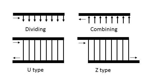
The flow in manifolds is extensively encountered in many industrial processes when it is necessary to distribute a large fluid stream into several parallel streams and then to collect them into one discharge stream, such as fuel cells, plate heat exchanger, radial flow reactor, and irrigation. Manifolds can usually be categorized into one of the following types: dividing, combining, Z-type and U-type manifolds (Fig. 1). A key question is the uniformity of the flow distribution and pressure drop.

Traditionally, most of theoretical models are based on Bernoulli equation after taking the frictional losses into account using a control volume (Fig. 2). The frictional loss is described using the Darcy–Weisbach equation. One obtains a governing equation of dividing flow as follows:

where

W is the velocity, P is the pressure, ρ is the density, D is the hydraulic diameter, f is the frictional coefficient, X is the axial coordinate in the manifold,

∆X = L/n. The n is the number of ports and L the length of the manifold (Fig. 2). This is fundamental of manifold and network models. Thus, a T-junction (Fig. 3) can be represented by two Bernoulli equations according to two flow outlets. A flow in manifold can be represented by a channel network model. A multi-scale parallel channel networks is usually described as the lattice network using analogy with the conventional electric circuit methods. A generalized model of the flow distribution in channel networks of planar fuel cells. Similar to Ohm's law, the pressure drop is assumed to be proportional to the flow rates. The relationship of pressure drop, flow rate and flow resistance is described as Q² = ∆P/R. f = 64/Re for laminar flow where Re is the Reynolds number. The frictional resistance, R = 128 μ L π d 4 using Poiseuille's law. Since they have same diameter and length in Fig. 3, their resistances are same, R₂ = R₃. Thus the velocities should be equal in two outlets or the flow rates should be equal according to the assumptions. Obviously this disobeys our observations. Our observations show that the greater the velocity (or momentum), the more fluid fraction through the straight direction. Only under very slow laminar flow, Q₂ may be equal to Q₃.

The question raised from the experiments by McNown and by Acrivos et al. Their experimental results showed a pressure rise after T-junction due to flow branching. This phenomenon was explained by Wang. Because of inertial effects, the fluid will prefer to the straight direction. Thus the flow rate of the straight pipe is greater than that of the vertical one. Furthermore, because the lower energy fluid in the boundary layer branches through the channels the higher energy fluid in the pipe centre remains in the pipe as shown in Fig. 4.

Thus, mass, momentum and energy conservations must be employed together for description of flow in manifolds. Wang recently carried out a series of studies of flow distribution in manifold systems. He unified main models into one theoretical framework and developed the most generalised model, based on the same control volume in Fig. 2. The governing equations can be obtained for the dividing, combining, U-type and Z-type arrangements. The Governing equation of the dividing flow:

or to a discrete equation:

In Eq.2, the inertial effects are corrected by a momentum factor, β. Eq.2b is a fundamental equation for most of discrete models. The equation can be solved by recurrence and iteration method for a manifold. It is clear that Eq.2a is limiting case of Eq.2b when ∆X → 0. Eq.2a is simplified to Eq.1 Bernoulli equation without the potential energy term when β=1 whilst Eq.2 is simplified to Kee’s model when β=0. Moreover, Eq.2 can be simplified to Acrivos et al.’s model after substituting Blasius’ equation, f = 0.3164 / R e 0.25 = f 0 W − 0.25 . Therefore, these main models are just a special case of Eq.2. Similarly, one can obtain the governing equations of the combining, U-type and Z-type arrangement.

The Governing equation of the combining flow:

or to a discrete equation:

The Governing equation of the U-type flow:

or to a discrete equation:

The Governing equation of the Z-type flow:

or to a discrete equation:

Eq.2 - Eq.5 are second order nonlinear ordinary differential equations for dividing, combining, U-type and Z-type manifolds, respectively. The second term in the left hand represents a frictional contribution known as the frictional term, and the third term does the momentum contribution as the momentum term. Their analytical solutions had been well-known challenges in this field for 50 years until 2008. Wang elaborated the most complete analytical solutions of Eq.2 - Eq.5. The present models have been extended into more complex configurations, such as single serpentine, multiple serpentine and straight parallel layout configurations, as shown in Fig. 5. Wang also established a direct, quantitative and systematic relationship between flow distribution, pressure drop, configurations, structures and flow conditions and developed an effective design procedures, measurements, criteria with characteristic parameters and guidelines on how to ensure uniformity of flow distribution as a powerful design tool.