
 | ||
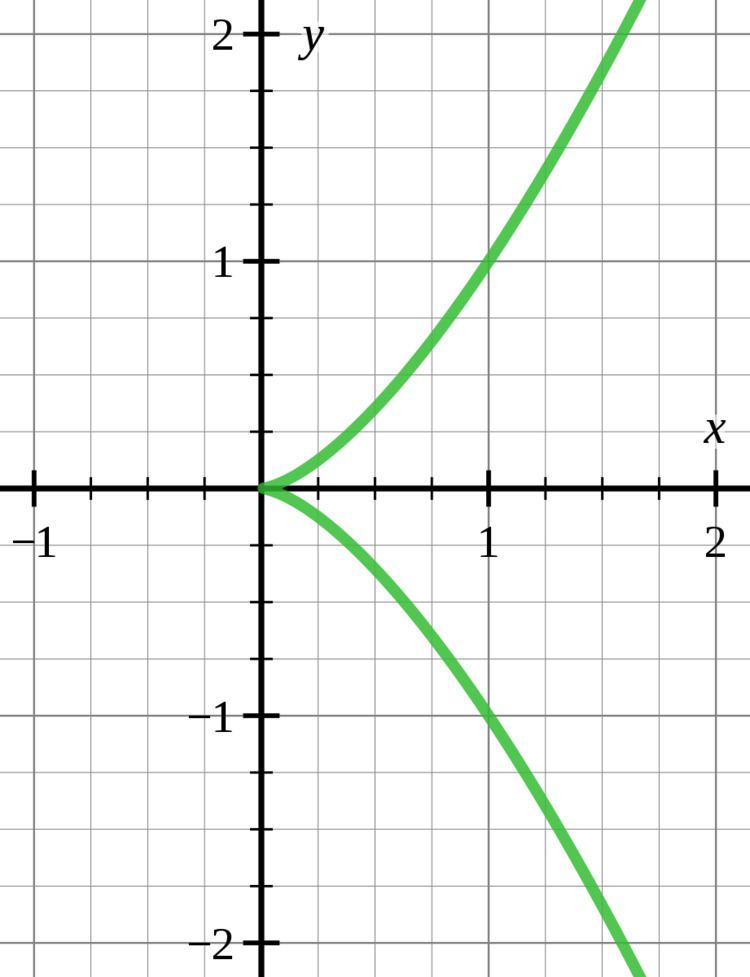
In mathematics a cusp, sometimes called spinode in old texts, is a point on a curve where a moving point on the curve must start to move backward. A typical example is given in the figure. A cusp is thus a type of singular point of a curve.
Contents
For a plane curve defined by a differentiable parametric equation
a cusp is a point where both derivatives of f and g are zero, and at least one of them changes sign. Cusps are local singularities in the sense that they involve only one value of the parameter t, contrarily to self-intersection points that involve several values.
For a curve defined by an implicit equation
cusps are points where the terms of lowest degree of the Taylor expansion of F are a power of a linear polynomial; however not all singular points that have this property are cusps. In some contexts, and in the remainder of this article, one restricts the definition of a cusp to the case where the non-zero part of lowest degree of the Taylor expansion of F has degree two.
A plane curve cusp may be put in one of the following forms by a diffeomorphism of the plane: x2 − y2k+1 = 0, where k ≥ 1 is an integer.
Classification in differential geometry
Consider a smooth real-valued function of two variables, say f(x, y) where x and y are real numbers. So f is a function from the plane to the line. The space of all such smooth functions is acted upon by the group of diffeomorphisms of the plane and the diffeomorphisms of the line, i.e. diffeomorphic changes of coordinate in both the source and the target. This action splits the whole function space up into equivalence classes, i.e. orbits of the group action.
One such family of equivalence classes is denoted by Ak±, where k is a non-negative integer. This notation was introduced by V. I. Arnold. A function f is said to be of type Ak± if it lies in the orbit of x2 ± yk+1, i.e. there exists a diffeomorphic change of coordinate in source and target which takes f into one of these forms. These simple forms x2 ± yk+1 are said to give normal forms for the type Ak±-singularities. Notice that the A2n+ are the same as the A2n− since the diffeomorphic change of coordinate (x,y) → (x, −y) in the source takes x2 + y2n+1 to x2 − y2n+1. So we can drop the ± from A2n± notation.
The cusps are then given by the zero-level-sets of the representatives of the A2n equivalence classes, where n ≥ 1 is an integer.
Examples
- Having a degenerate quadratic part, i.e. the quadratic terms in the Taylor series of f form a perfect square, say L(x, y)2, where L(x, y) is linear in x and y, and
- L(x, y) does not divide the cubic terms in the Taylor series of f(x, y).
For a type A4-singularity we need f to have a degenerate quadratic part (this gives type A≥2), that L does divide the cubic terms (this gives type A≥3), another divisibility condition (giving type A≥4), and a final non-divisibility condition (giving type exactly A4).
To see where these extra divisibility conditions come from, assume that f has a degenerate quadratic part L2 and that L divides the cubic terms. It follows that the third order taylor series of f is given by L2 ± LQ where Q is quadratic in x and y. We can complete the square to show that L2 ± LQ = (L ± ½Q)2 – ¼Q4. We can now make a diffeomorphic change of variable (in this case we simply substitute polynomials with linearly independent linear parts) so that (L ± ½Q)2 − ¼Q4 → x12 + P1 where P1 is quartic (order four) in x1 and y1. The divisibility condition for type A≥4 is that x1 divides P1. If x1 does not divide P1 then we have type exactly A3 (the zero-level-set here is a tacnode). If x1 divides P1 we complete the square on x12 + P1 and change coordinates so that we have x22 + P2 where P2 is quintic (order five) in x2 and y2. If x2 does not divide P2 then we have exactly type A4, i.e. the zero-level-set will be a rhamphoid cusp.
Applications
Cusps appear naturally when projecting into a plane a smooth curve in the three dimensional Euclidean space. In general, such a projection is a curve whose singularities are self-crossing points and ordinary cusps. Self-crossing points appear when two different points of the curves have the same projection. Ordinary cusps appear when the tangent to the curve is parallel to the direction of projection (that is when the tangent projects on a single point). More complicated singularities occur when several phenomena occurs simultaneously. For example, rhamphoid cusps occur for inflection points (and for undulation points) for which the tangent is parallel to the direction of projection.
In many cases, and typically in computer vision and computer graphics, the curve that is projected is the curve of the critical points of the restriction to a (smooth) spatial object of the projection. A cusp appears thus as a singularity of the contour of the image of the object (vision) or of its shadow (computer graphics).
Caustics and wave fronts are other examples of curves having cusps that are visible in the real world.