
 | ||
Collocation is a procedure used in remote sensing to match measurements from two or more different instruments. This is done for two main reasons: for validation purposes when comparing measurements of the same variable, and to relate measurements of two different variables either for performing retrievals or for prediction. In the second case the data is later fed into some type of statistical inverse method such as a neural network, statistical classification algorithm, kernel estimator or a linear least squares. In principle, most collocation problems can be solved by a nearest neighbor search, but in practice there are many other considerations involved and the best method is highly specific to the particular matching of instruments. Here we deal with some of the most important considerations along with specific examples.
Contents
There are at least two main considerations when performing collocations. The first is the sampling pattern of the instrument. Measurements may be dense and regular, such as those from a cross-track scanning satellite instrument. In this case, some form of interpolation may be appropriate. On the other hand, the measurements may be sparse, such as a one-off field campaign designed for some particular validation exercise. The second consideration is the instrument footprint, which can range from something approaching a point measurement such as that of a radiosonde, or it might be several kilometers in diameter such as that of a satellite-mounted, microwave radiometer. In the latter case, it is appropriate to take into account the instrument antenna pattern when making comparisons with another instrument having both a smaller footprint and a denser sampling, that is, several measurements from the one instrument will fit into the footprint of the other.
Just as the instrument has a spatial footprint, it will also have a temporal footprint, often called the integration time. While the integration time is usually less than a second, which for meteorological applications is essentially instantaneous, there are many instances where some form of time averaging can considerably ease the collocation process.
The collocations will need to be screened based on both the time and length scales of the phenomenon of interest. This will further facilitate the collocation process since remote sensing and other measurement data is almost always binned in some way. Certain atmospheric phenomena such as clouds or convection are quite transient so that we need not consider collocations with a time error of more than an hour or so. Sea ice, on the other hand, moves and evolves quite slowly, so that measurements separated by as much as a day or more might still be useful.
Satellites
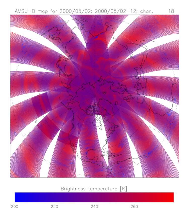
The satellites that most concern us are those with a low-Earth, polar orbit since geostationary satellites view the same point throughout their lifetime. The diagram shows measurements from AMSU-B instruments mounted on three satellites over a period of 12 hours. This illustrates both the orbit path and the scan pattern which runs crosswise. Since the orbit of a satellite is deterministic, barring orbit maneuvers, we can predict the location of the satellite at a given time and, by extension, the location of the measurement pixels. In theory, collocations can be performed by inverting the determining equations starting from the desired time period. In practice, partially processed data (usually referred to as level 1b, 1c or level 2) contain the coordinates of each of the measurement pixels and it is common to simply feed these coordinates to a nearest neighbor search. As mentioned previously, the satellite data is always binned in some manner. At minimum, the data will be arranged in swaths extending from pole to pole. The swaths will be labelled by time period and the approximate location known.
Radiosondes
Radiosondes are particularly important for collocation studies because they measure atmospheric variables more accurately and more directly than satellite or other remote-sensing instruments. In addition, radiosonde samples are effectively instantaneous point measurements. One issue with radiosondes carried aloft by weather balloons is balloon drift. In, this is handled by averaging all the satellite pixels within a 50 km radius of the balloon launch.
If high-resolution sonde data, which normally has a constant sampling rate or includes the measurement time, is used, then the lateral motion can be traced from the wind data. Even with low-resolution data, the motion can still be approximated by assuming a constant ascent rate. Excepting a short bit towards the end, the linear ascent can be clearly seen in the figure above. We can show that the ascent rate of a balloon is given by the following equation
where g is gravitational acceleration, k relates the height, h, and surface area, A, of the balloon to its volume: V = khA; Rs is the equivalent "gas constant" of the balloon, Ra is the gas constant of the air and cD is the drag coefficient of the balloon. Substituting some sensible values for each of the constants, k=1. (the balloon is a perfect cylinder), h=2. m, cD = 1. and Ra is the gas constant of helium, returns an ascent rate of 4.1 m/s. Compare this with the values shown in the histogram which compiles all of the radiosonde launches from the Polarstern research vessel over a period of eleven years between 1992 and 2003.
Interpolation
For gridded data such as assimilation or reanalysis data, interpolation is likely the most appropriate method for performing any type of comparison. A specific point in both physical position and time is easy to locate within the grid and interpolation performed between the nearest neighbors. Linear interpolation (bilinear, trilinear etc.) is the most common, though cubic is used as well but is probably not worth the extra computational overhead. If the variable of interest has a relatively smooth rate of change (temperature is a good example of this because it has a diffusion mechanism, radiative transfer, not available to other atmospheric variables), then interpolation can eliminate much of the error associated with collocation.
Interpolation may also be appropriate for many types of satellite instruments, for instance a cross-track scanning instrument like Landsat. In data derived from the Advanced Microwave Sounding Unit (AMSU) are interpolated (although not for the purposes of collocation) using a slight variation of trilinear interpolation. Since measurements within a single scan track are laid out in an approximately rectangular grid, bilinear interpolation can be performed. By searching for the nearest overlapping scan track both forwards and backwards in time, the spatial interpolates can then be interpolated in time. This technique works better with derived quantities rather than raw brightness temperatures since the scan angle will already have been accounted for.
For instruments with a more irregular sampling pattern, such as the Advanced Microwave Scanning Radiometer-EOS (AMSR-E) instrument which has a circular scanning pattern, we need a more general form of interpolation such as kernel estimation. A method commonly used for this particular instrument, as well as SSM/I, is a simple daily average within regularly gridded, spatial bins .
Trajectories
To collocate measurements of a medium- to long-lived atmospheric tracer with a second instrument, running trajectories can considerably improve the accuracy. It also simplifies the analysis somewhat: a trajectory is run both forwards and backwards from the measurement location and between the desired time window. Note that the acceptable time window has now become longer because the error from transport induced changes in the tracer is removed: the tracer lifetime would be a good window to use. Since the trajectories provide a location for every point in time within the time window, there is no need to check multiple measurements from the second instrument. Every time within the trajectory is checked for the distance criterion but within a very narrow window. Alternatively, the exact times of the measurements for the second instrument are interpolated within the trajectory. Only the smallest distance error below the threshold is used and the distance criterion can be made smaller as a consequence.
Example: Pol-Ice Campaign
Collocations of sea ice thickness and brightness temperatures taken during the Pol-Ice Campaign are an excellent example since they illustrate many of the most important principles as well as demonstrating the necessity of taking into account the individual case. The Pol-Ice campaign was conducted in the N. Baltic in March 2007 as part of the SMOS-Ice project in preparation for the launch of the Soil Moisture and Ocean Salinity satellite. Because of the low frequency of the SMOS instrument, it is hoped that it will render information on sea ice thickness, therefore the campaign comprised measurements of both sea ice thickness and emitted brightness temperature. Brightness temperatures were measured with the EMIRAD L-band microwave radiometer carried on board an airplane. Ice thickness was measured with the E-M Bird ice thickness meter which was carried by a helicopter. The E-M Bird measures ice thickness with a combination of inductance measurements to determine the location of the ice-water interface and a laser altimeter to measure the height of the ice surface. The map above shows the flight tracks of both instruments which were approximately coincident but obviously subject to pilot error.
Since the flight paths of both aircraft were approximately linear, the first step in the collocation process was to convert all the coincident flights to Cartesian coordinates with the x-axis being lateral distance and the y-axis transverse distance. In this way, collocations can be performed in two ways: crudely, by matching only the x distances, and more precisely by matching both coordinates.
More importantly, the footprint size of the radiometer is many times larger than that of the E-M Bird meter. The figure to the left shows the antenna response function for the radiometer. The full width at half maximum is 31 degrees. Since the aircraft was flying at approximately 500 m, this translates to a footprint size of 200 m or more. Meanwhile, the footprint size of the E-M Bird was roughly 40 m with a sample spacing of only 2 to 4 m. Rather than looking to nearest neighbors, which would have produced poor results, a weighted average of the thickness measurements was performed for each radiometer measurement. Weights were calculated based on the radiometer response function which is almost a perfect Gaussian up to about 45 degrees. Points could be excluded based on distance along the flight path. For validation of sea ice emissivity forward model calculations, this was further refined by performing an emissivity calculation for each thickness measurement and averaging over the radiometer footprint.
The figure below illustrates relative measurement locations from each of the instruments used in the Pol-Ice campaign. Two overpasses are shown: one from the airplane carrying the EMIRAD radiometer and one from the helicopter carrying the E-M Bird instrument. The x-axis is along the line of the flight path. EMIRAD footprints are drawn with lines, E-M Bird inductance measurements are represented by circles and LIDAR measurements with dots.