Biham–Middleton–Levine traffic model

History

The Biham–Middleton–Levine traffic model was first formulated by Ofer Biham, A. Alan Middleton, and Dov Levine in 1992. Biham et al found that as the density of traffic increased, the steady-state flow of traffic suddenly went from smooth flow to a complete jam. In 2005, Raissa D'Souza found that for some traffic densities, there is an intermediate phase characterized by periodic arrangements of jams and smooth flow. In the same year, Angel, Holroyd and Martin were the first to rigorously prove that for densities close to one, the system will always jam. Later, in 2006, Tim Austin and Itai Benjamini found that for a square lattice of side N, the model will always self-organize to reach full speed if there are fewer than N/2 cars.

Lattice space

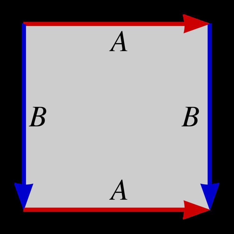
The cars are typically placed on a square lattice that is topologically equivalent to a torus: that is, cars that move off the right edge would reappear on the left edge; and cars that move off the bottom edge would reappear on the top edge.

There has also been research in rectangular lattices instead of square ones. For rectangles with coprime dimensions, the intermediate states are self-organized bands of jams and free-flow with detailed geometric structure, that repeat periodically in time. In non-coprime rectangles, the intermediate states are typically disordered rather than periodic.

Phase transitions

Despite the simplicity of the model, it has two highly distinguishable phases – the jammed phase, and the free-flowing phase. For low numbers of cars, the system will usually organize itself to achieve a smooth flow of traffic. In contrast, if there is a high number of cars, the system will become jammed to the extent that no single car will move. Typically, in a square lattice, the transition density is when there are around 32% as many cars as there are possible spaces in the lattice.

Intermediate phase

The intermediate phase occurs close to the transition density, combining features from both the jammed and free-flowing phases. There are principally two intermediate phases – disordered (which could be meta-stable) and periodic (which are provably stable). On rectangular lattices with coprime dimensions, only periodic orbits exist. In 2008 periodic intermediate phases were also observed in square lattices. Yet, on square lattices disordered intermediate phases are more frequently observed and tend to dominate densities close to the transition region.

Rigorous analysis

Despite the simplicity of the model, rigorous analysis is very nontrivial. Nonetheless, there have been mathematical proofs regarding the Biham–Middleton–Levine traffic model. Proofs so far have been restricted to the extremes of traffic density. In 2005, Alexander Holroyd et al proved that for densities close to one, the system will always jam. In 2006, Tim Austin and Itai Benjamini proved that the model will always reach the free-flowing phase if the number of cars is less than half the edge length for a square lattice.

It would be ideal to formulate a rigorous method to predict the end result of any starting position, especially in the intermediate phases. To that end, this model has been the subject of research for several scientists.

Non-orientable surfaces

The model is typically studied on the orientable torus, but it is possible to implement the lattice on a Klein bottle. When the red cars reach the right edge, they reappear on the left edge except flipped vertically; the ones at the bottom are now at the top, and vice versa. More formally, for every y ∈ { 0 , … , N − 1 } , a red car exiting the site ( N − 1 , y ) would enter the site ( 0 , N − y − 1 ) . It is also possible to implement it on the real projective plane. In addition to flipping the red cars, the same is done for the blue cars: for every x ∈ { 0 , … , N − 1 } , a blue car exiting the site ( x , N − 1 ) would enter the site ( N − x − 1 , 0 ) .

The behaviour of the system on the Klein bottle is much more similar to the one on the torus than the one on the real projective plane. For the Klein bottle setup, the mobility as a function of density starts to decrease slightly sooner than in the torus case, although the behaviour is similar for densities greater than the critical point. The mobility on the real projective plane, decreases more gradually for densities from zero to the critical point. In the real projective plane, local jams may form at the corners of the lattice even though the rest of the lattice is free-flowing.

Randomization

A randomized variant of the BML traffic model, called BML-R, was studied in 2010. Under periodic boundaries, instead of updating all cars of the same colour at once during each step, the randomized model performs L 2 updates (where L is the side length of the presumably square lattice): each time, a random cell is selected and, if it contains a car, it is moved to the next cell if possible. In this case, the intermediate state observed in the usual BML traffic model does not exist, due to the non-deterministic nature of the randomized model; instead the transition from the jammed phase to the free flowing phase is sharp.

Under open boundary conditions, instead of having cars that drive off one edge wrapping around the other side, new cars are added on the left and top edges with probability α and removed from the right and bottom edges β respectively. In this case, the number of cars in the system can change over time, and local jams can cause the lattice to appear very different from the usual model, such as having coexistence of jams and free-flowing areas; containing large empty spaces; or containing mostly cars of one type.