Bayes' theorem

Statement of theorem

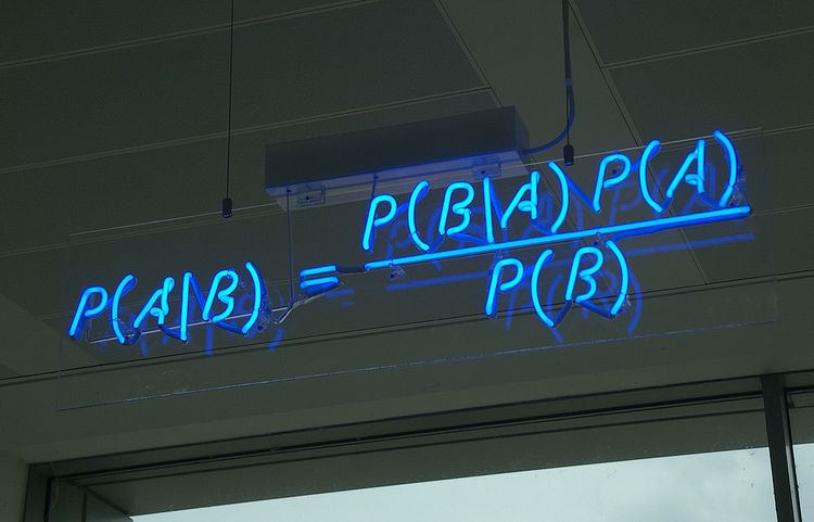
Bayes' theorem is stated mathematically as the following equation:

P ( A ∣ B ) = P ( B ∣ A ) P ( A ) P ( B ) ,

where A and B are events and P(B) ≠ 0.

P(A) and P(B) are the probabilities of observing A and B without regard to each other.

P(A | B), a conditional probability, is the probability of observing event A given that B is true.

P(B | A) is the probability of observing event B given that A is true.

History

Bayes’ theorem was named after the Reverend Thomas Bayes (1701–1761), who studied how to compute a distribution for the probability parameter of a binomial distribution (in modern terminology). Bayes’ unpublished manuscript was significantly edited by Richard Price before it was posthumously read at the Royal Society. Price edited Bayes’ major work “An Essay towards solving a Problem in the Doctrine of Chances” (1763), which appeared in “Philosophical Transactions,” and contains Bayes’ Theorem. Price wrote an introduction to the paper which provides some of the philosophical basis of Bayesian statistics. In 1765 he was elected a Fellow of the Royal Society in recognition of his work on the legacy of Bayes.

The French mathematician Pierre-Simon Laplace reproduced and extended Bayes’ results in 1774, apparently quite unaware of Bayes’ work. The Bayesian interpretation of probability was developed mainly by Laplace.

Stephen Stigler suggested in 1983 that Bayes’ theorem was discovered by Nicholas Saunderson, a blind English mathematician, some time before Bayes; that interpretation, however, has been disputed. Martyn Hooper and Sharon McGrayne have argued that Richard Price's contribution was substantial:

By modern standards, we should refer to the Bayes–Price rule. Price discovered Bayes’ work, recognized its importance, corrected it, contributed to the article, and found a use for it. The modern convention of employing Bayes’ name alone is unfair but so entrenched that anything else makes little sense.

Drug testing

Suppose a drug test is 99% sensitive and 99% specific. That is, the test will produce 99% true positive results for drug users and 99% true negative results for non-drug users. Suppose that 0.5% of people are users of the drug. If a randomly selected individual tests positive, what is the probability that he is a user?

P ( User ∣ + ) = P ( + ∣ User ) P ( User ) P ( + ∣ User ) P ( User ) + P ( + ∣ Non-user ) P ( Non-user ) = 0.99 × 0.005 0.99 × 0.005 + 0.01 × 0.995 ≈ 33.2 %

Despite the apparent accuracy of the test, if an individual tests positive, it is more likely that they do not use the drug than that they do. This surprising result arises because the number of non-users is very large compared to the number of users; thus the number of false positives outweighs the number of true positives. To use concrete numbers, if 1000 individuals are tested, there are expected to be 995 non-users and 5 users. From the 995 non-users, 0.01 × 995 ≃ 10 false positives are expected. From the 5 users, 0.99 × 5 ≃ 5 true positives are expected. Out of 15 positive results, only 5, about 33%, are genuine. This illustrates the importance of base rates, and how the formation of policy can be egregiously misguided if base rates are neglected.

The importance of specificity in this example can be seen by calculating that even if sensitivity is raised to 100% and specificity remains at 99% then the probability of the person being a drug user only rises from 33.2% to 33.4%, but if the sensitivity is held at 99% and the specificity is increased to 99.5% then probability of the person being a drug user rises to about 49.9%.

A more complicated example

The entire output of a factory is produced on three machines. The three machines account for 20%, 30%, and 50% of the output, respectively. The fraction of defective items produced is this: for the first machine, 5%; for the second machine, 3%; for the third machine, 1%. If an item is chosen at random from the total output and is found to be defective, what is the probability that it was produced by the third machine?

A solution is as follows. Let A_i denote the event that a randomly chosen item was made by the ith machine (for i = 1,2,3). Let B denote the event that a randomly chosen item is defective. Then, we are given the following information:

P(A₁) = 0.2,    P(A₂) = 0.3,    P(A₃) = 0.5.

If the item was made by the first machine, then the probability that it is defective is 0.05; that is, P(B | A₁) = 0.05. Overall, we have

P(B | A₁) = 0.05,    P(B | A₂) = 0.03,    P(B | A₃) = 0.01.

To answer the original question, we first find P(B). That can be done in the following way:

P(B) = Σ_i P(B | A_i) P(A_i) = (0.05)(0.2) + (0.03)(0.3) + (0.01)(0.5) = 0.024.

Hence 2.4% of the total output of the factory is defective.

We are given that B has occurred, and we want to calculate the conditional probability of A₃. By Bayes' theorem,

P(A₃ | B) = P(B | A₃) P(A₃)/P(B) = (0.01)(0.50)/(0.024) = 5/24.

Given that the item is defective, the probability that it was made by the third machine is only 5/24. Although machine 3 produces half of the total output, it produces a much smaller fraction of the defective items. Hence the knowledge that the item selected was defective enables us to replace the prior probability P(A₃) = 1/2 by the smaller posterior probability P(A₃ | B) = 5/24.

Once again, the answer can be reached without recourse to the formula by applying the conditions to any hypothetical number of cases. For example, in 100,000 items produced by the factory, 20,000 will be produced by Machine A, 30,000 by Machine B, and 50,000 by Machine C. Machine A will produce 1000 defective items, Machine B 900, and Machine C 500. Of the total 2400 defective items, only 500, or 5/24 were produced by Machine C.

Interpretations

The interpretation of Bayes’ theorem depends on the interpretation of probability ascribed to the terms. The two main interpretations are described below.

Bayesian interpretation

In the Bayesian (or epistemological) interpretation, probability measures a “degree of belief.” Bayes’ theorem then links the degree of belief in a proposition before and after accounting for evidence. For example, suppose it is believed with 50% certainty that a coin is twice as likely to land heads than tails. If the coin is flipped a number of times and the outcomes observed, that degree of belief may rise, fall or remain the same depending on the results.

For proposition A and evidence B,

P (A ), the prior, is the initial degree of belief in A.

P (A | B ), the “posterior,” is the degree of belief having accounted for B.

the quotient P(B |A )/P(B) represents the support B provides for A.

For more on the application of Bayes’ theorem under the Bayesian interpretation of probability, see Bayesian inference.

Frequentist interpretation

In the frequentist interpretation, probability measures a “proportion of outcomes.” For example, suppose an experiment is performed many times. P(A) is the proportion of outcomes with property A, and P(B) that with property B. P(B | A ) is the proportion of outcomes with property B out of outcomes with property A, and P(A | B ) the proportion of those with A out of those with B.

The role of Bayes’ theorem is best visualized with tree diagrams, as shown to the right. The two diagrams partition the same outcomes by A and B in opposite orders, to obtain the inverse probabilities. Bayes’ theorem serves as the link between these different partitionings.

Example

An entomologist spots what might be a rare subspecies of beetle, due to the pattern on its back. In the rare subspecies, 98% have the pattern, or P(Pattern | Rare) = 98%. In the common subspecies, 5% have the pattern. The rare subspecies accounts for only 0.1% of the population. How likely is the beetle having the pattern to be rare, or what is P(Rare | Pattern)?

From the extended form of Bayes’ theorem (since any beetle can be only rare or common),

P ( Rare ∣ Pattern ) = P ( Pattern ∣ Rare ) P ( Rare ) P ( Pattern ∣ Rare ) P ( Rare ) + P ( Pattern ∣ Common ) P ( Common ) = 0.98 × 0.001 0.98 × 0.001 + 0.05 × 0.999 ≈ 1.9 %

Simple form

For events A and B, provided that P(B) ≠ 0,

P ( A ∣ B ) = P ( B ∣ A ) P ( A ) P ( B ) ⋅

In many applications, for instance in Bayesian inference, the event B is fixed in the discussion, and we wish to consider the impact of its having been observed on our belief in various possible events A. In such a situation the denominator of the last expression, the probability of the given evidence B, is fixed; what we want to vary is A. Bayes’ theorem then shows that the posterior probabilities are proportional to the numerator:

P ( A ∣ B ) ∝ P ( A ) ⋅ P ( B ∣ A )   (proportionality over A for given B).

In words: posterior is proportional to prior times likelihood.

If events A₁, A₂, ..., are mutually exclusive and exhaustive, i.e., one of them is certain to occur but no two can occur together, and we know their probabilities up to proportionality, then we can determine the proportionality constant by using the fact that their probabilities must add up to one. For instance, for a given event A, the event A itself and its complement ¬A are exclusive and exhaustive. Denoting the constant of proportionality by c we have

P ( A ∣ B ) = c ⋅ P ( A ) ⋅ P ( B ∣ A )  and  P ( ¬ A ∣ B ) = c ⋅ P ( ¬ A ) ⋅ P ( B ∣ ¬ A ) .

Adding these two formulas we deduce that

1 = c ⋅ ( P ( B ∣ A ) ⋅ P ( A ) + P ( B ∣ ¬ A ) ⋅ P ( ¬ A ) ) ,

or

c = 1 P ( B ∣ A ) ⋅ P ( A ) + P ( B ∣ ¬ A ) ⋅ P ( ¬ A ) = 1 P ( B ) .

Alternative form

Another form of Bayes’ Theorem that is generally encountered when looking at two competing statements or hypotheses is:

P ( A ∣ B ) = P ( B ∣ A ) P ( A ) P ( B ∣ A ) P ( A ) + P ( B ∣ ¬ A ) P ( ¬ A ) ⋅

For an epistemological interpretation:

For proposition A and evidence or background B,

P(A),the prior probability, is the initial degree of belief in A.

P(−A), is the corresponding probability of the initial degree of belief against A: 1 − P(A) = P(−A)

P(B | A), the conditional probability or likelihood, is the degree of belief in B, given that the proposition A is true.

P(B | −A), the conditional probability or likelihood, is the degree of belief in B, given that the proposition A is false.

P(A | B), the posterior probability, is the probability for A after taking into account B for and against A.

Extended form

Often, for some partition {A_j} of the sample space, the event space is given or conceptualized in terms of P(A_j) and P(B | A_j). It is then useful to compute P(B) using the law of total probability:

P ( B ) = ∑ j P ( B ∣ A j ) P ( A j ) , ⇒ P ( A i ∣ B ) = P ( B ∣ A i ) P ( A i ) ∑ j P ( B ∣ A j ) P ( A j ) ⋅

In the special case where A is a binary variable:

P ( A ∣ B ) = P ( B ∣ A ) P ( A ) P ( B ∣ A ) P ( A ) + P ( B ∣ ¬ A ) P ( ¬ A ) ⋅

Random variables

Consider a sample space Ω generated by two random variables X and Y. In principle, Bayes’ theorem applies to the events A = {X = x} and B = {Y = y}. However, terms become 0 at points where either variable has finite probability density. To remain useful, Bayes’ theorem may be formulated in terms of the relevant densities (see Derivation).

Simple form

If X is continuous and Y is discrete,

f X ( x ∣ Y = y ) = P ( Y = y ∣ X = x ) f X ( x ) P ( Y = y ) .

If X is discrete and Y is continuous,

P ( X = x ∣ Y = y ) = f Y ( y ∣ X = x ) P ( X = x ) f Y ( y ) .

If both X and Y are continuous,

f X ( x ∣ Y = y ) = f Y ( y ∣ X = x ) f X ( x ) f Y ( y ) .

Extended form

A continuous event space is often conceptualized in terms of the numerator terms. It is then useful to eliminate the denominator using the law of total probability. For f_Y(y), this becomes an integral:

f Y ( y ) = ∫ − ∞ ∞ f Y ( y ∣ X = ξ ) f X ( ξ ) d ξ .

Bayes’ rule

Bayes' rule is Bayes’ theorem in odds form.

O ( A 1 : A 2 ∣ B ) = O ( A 1 : A 2 ) ⋅ Λ ( A 1 : A 2 ∣ B )

where

Λ ( A 1 : A 2 ∣ B ) = P ( B ∣ A 1 ) P ( B ∣ A 2 )

is called the Bayes factor or likelihood ratio and the odds between two events is simply the ratio of the probabilities of the two events. Thus

O ( A 1 : A 2 ) = P ( A 1 ) P ( A 2 ) , O ( A 1 : A 2 ∣ B ) = P ( A 1 ∣ B ) P ( A 2 ∣ B ) ,

So the rule says that the posterior odds are the prior odds times the Bayes factor, or in other words, posterior is proportional to prior times likelihood.

For events

Bayes’ theorem may be derived from the definition of conditional probability:

P ( A ∣ B ) = P ( A ∩ B ) P ( B ) ,  if  P ( B ) ≠ 0 , P ( B ∣ A ) = P ( A ∩ B ) P ( A ) ,  if  P ( A ) ≠ 0 , ⇒ P ( A ∩ B ) = P ( A ∣ B ) P ( B ) = P ( B ∣ A ) P ( A ) , ⇒ P ( A ∣ B ) = P ( B ∣ A ) P ( A ) P ( B ) ,  if  P ( B ) ≠ 0.

For random variables

For two continuous random variables X and Y, Bayes’ theorem may be analogously derived from the definition of conditional density:

f X ( x ∣ Y = y ) = f X , Y ( x , y ) f Y ( y ) f Y ( y ∣ X = x ) = f X , Y ( x , y ) f X ( x ) ⇒ f X ( x ∣ Y = y ) = f Y ( y ∣ X = x ) f X ( x ) f Y ( y ) .